Alerts v6The strategy includes:
✅ EMA-based trend direction (fast vs slow)
✅ RSI filtering for overbought/oversold control
✅ ADX confirmation for strong trend validation
✅ Pullback & BOS detection for precision entries
✅ Per-bar change logic for adaptive entry timing
✅ Session/day gating to control trading hours
✅ JSON alert integration for AI trading bots or webhooks
This script is Pine Script v6 compatible and optimized for automated alert-based trading setups such as AI trading bots, webhook systems, and VPS-linked executions.
Recommended Timeframes: 5m, 15m, 30m
Markets: XAUUSD, FX pairs, indices, and metals
Cerca negli script per "the strat"

Systematic Investment Tracker by Ceyhun Gonul### English Description
**Systematic Investment Tracker with Enhanced Features**
This script, titled **Systematic Investment Tracker with Enhanced Features**, is a TradingView tool designed to support systematic investments across different market conditions. It provides traders with two customizable investment strategies — **Continuous Buying** and **Declining Buying** — and includes advanced dynamic investment adjustment features for each.
#### Detailed Explanation of Script Features and Originality
1. **Two Investment Strategies**:
- **Continuous Buying**: This strategy performs purchases consistently at each interval, as set by the user, regardless of market price changes. It follows the principle of dollar-cost averaging, allowing users to build an investment position over time.
- **Declining Buying**: Unlike Continuous Buying, this strategy triggers purchases only when the asset's price has declined from the previous interval's closing price. This approach helps users capitalize on lower price points, potentially improving average costs during downward trends.
2. **Dynamic Investment Adjustment**:
- For both strategies, the script includes a **Dynamic Investment Adjustment** feature. If enabled, this feature increases the purchasing amount by 50% if the current price has fallen by a specific user-defined percentage relative to the previous price. This allows users to accumulate a larger position when the asset is declining, which may benefit long-term cost-averaging strategies.
3. **Customizable Time Frames**:
- Users can specify a **start and end date** for investment, allowing them to restrict or backtest strategies within a specific timeframe. This feature is valuable for evaluating strategy performance over specific market cycles or historical periods.
4. **Graphical Indicators and Labels**:
- The script provides graphical labels on the chart that display purchase points. These indicators help users visualize their investment entries based on the strategy selected.
- A summary **performance label** is also displayed, providing real-time updates on the total amount spent, accumulated quantity, average cost, portfolio value, and profit percentage for each strategy.
5. **Language Support**:
- The script includes English and Turkish language options. Users can toggle between these languages, allowing the summary label text and descriptions to be displayed in their preferred language.
6. **Performance Comparison Table**:
- An optional **Performance Comparison Table** is available, offering a side-by-side analysis of net profit, total investment, and profit percentage for both strategies. This comparison table helps users assess which strategy has yielded better returns, providing clarity on each approach's effectiveness under the chosen parameters.
#### How the Script Works and Its Uniqueness
This closed-source script brings together two established investment strategies in a single, dynamic tool. By integrating continuous and declining purchase strategies with advanced settings for dynamic investment adjustment, the script offers a powerful, flexible tool for both passive and active investors. The design of this script provides unique benefits:
- Enables automated, systematic investment tracking, allowing users to build positions gradually.
- Empowers users to leverage declines through dynamic adjustments to optimize average cost over time.
- Presents an easy-to-read performance label and table, enabling an efficient and transparent performance comparison for informed decision-making.
---
### Türkçe Açıklama
**Gelişmiş Özellikli Sistematik Yatırım Takipçisi**
**Gelişmiş Özellikli Sistematik Yatırım Takipçisi** adlı bu TradingView scripti, çeşitli piyasa koşullarında sistematik yatırım stratejilerini desteklemek üzere tasarlanmış bir araçtır. Script, kullanıcıya iki özelleştirilebilir yatırım stratejisi — **Sürekli Alım** ve **Düşen Alım** — ve her strateji için gelişmiş dinamik yatırım ayarlama seçenekleri sunar.
#### Script Özelliklerinin Detaylı Açıklaması ve Özgünlük
1. **İki Yatırım Stratejisi**:
- **Sürekli Alım**: Bu strateji, fiyat değişimlerine bakılmaksızın kullanıcının belirlediği her aralıkta sabit bir miktar yatırım yapar. Bu yaklaşım, uzun vadede pozisyonu kademeli olarak oluşturmak isteyenler için idealdir.
- **Düşen Alım**: Sürekli Alım’ın aksine, bu strateji yalnızca fiyat bir önceki aralığın kapanış fiyatına göre düştüğünde alım yapar. Bu yöntem, yatırımcıların daha düşük fiyatlardan alım yaparak ortalama maliyeti potansiyel olarak iyileştirmelerine yardımcı olur.
2. **Dinamik Yatırım Ayarlaması**:
- Her iki strateji için de **Dinamik Yatırım Ayarlaması** özelliği bulunmaktadır. Bu özellik aktif edildiğinde, mevcut fiyatın bir önceki fiyata göre kullanıcı tarafından belirlenen bir yüzde oranında düşmesi durumunda alım miktarını %50 artırır. Bu durum, uzun vadede maliyet ortalaması stratejilerine katkıda bulunur.
3. **Özelleştirilebilir Tarih Aralığı**:
- Kullanıcılar, yatırımı belirli bir tarih aralığında sınırlandırmak veya test etmek için bir **başlangıç ve bitiş tarihi** belirleyebilir. Bu özellik, strateji performansını geçmiş piyasa döngüleri veya belirli dönemlerde değerlendirmek için kullanışlıdır.
4. **Grafiksel İşaretleyiciler ve Etiketler**:
- Script, grafik üzerinde alım noktalarını gösteren işaretleyiciler sağlar. Bu görsel göstergeler, kullanıcıların seçilen stratejiye göre yatırım girişlerini görselleştirmesine yardımcı olur.
- Ayrıca, her strateji için harcanan toplam tutar, biriken miktar, ortalama maliyet, portföy değeri ve kâr yüzdesi gibi bilgileri gerçek zamanlı olarak gösteren bir **performans etiketi** sunar.
5. **Dil Desteği**:
- Script, İngilizce ve Türkçe dillerini desteklemektedir. Kullanıcılar, performans etiketi metninin ve açıklamalarının tercih ettikleri dilde görüntülenmesi için dil seçimini yapabilir.
6. **Performans Karşılaştırma Tablosu**:
- İsteğe bağlı olarak kullanılabilen bir **Performans Karşılaştırma Tablosu**, her iki strateji için net kâr, toplam yatırım ve kâr yüzdesi gibi bilgileri yan yana analiz eder. Bu tablo, kullanıcıların hangi stratejinin daha yüksek getiri sağladığını değerlendirmesine yardımcı olur.
#### Scriptin Çalışma Prensibi ve Özgünlüğü
Bu script, iki yatırım stratejisini gelişmiş bir araçta birleştirir. Sürekli ve düşen fiyatlara dayalı alım stratejilerini dinamik yatırım ayarlama özelliğiyle entegre ederek yatırımcılar için güçlü ve esnek bir çözüm sunar. Script’in tasarımı aşağıdaki benzersiz faydaları sağlamaktadır:
- Otomatik, sistematik yatırım takibi yaparak kullanıcıların pozisyonlarını kademeli olarak oluşturmalarına olanak tanır.
- Dinamik ayarlama ile düşüşlerden yararlanarak zaman içinde ortalama maliyeti optimize etme olanağı sağlar.
- Her iki stratejinin performansını basit ve anlaşılır bir şekilde karşılaştıran etiket ve tablo ile verimli bir performans değerlendirmesi sunar.

Velocity And Acceleration with Strategy: Traders Magazine◙ OVERVIEW
Hi, Ivestors and Traders... This Indicator, the focus is Scott Cong's article in the Stocks & Commodities September issue, “VAcc: A Momentum Indicator Based On Velocity And Acceleration”. I have also added a trading strategy for you to benefit from this indicator. First of all, let's look at what the indicator offers us and what its logic is. First, let's focus on the logic of the strategy.
◙ CONCEPTS
Here is a new indicator based on some simple physics concepts that is easy to use, responsive and precise. Learn how to calculate and use it.
The field of physics gives us some important principles that are highly applicable to analyzing the markets. In this indicator, I will present a momentum indicator. Scott Cong developed based on the concepts of velocity and acceleration this indicator. Of the many characteristics of price that traders and analysts often study, rate and rate of change are useful ones. In other words, it’s helpful to know: How fast is price moving, and is it speeding up or slowing down? How is price changing from one period to the next? The indicator I’m introducing here is calculated using the current bar (C) and every bar of a lookback period from the current bar. He named the indicator the VAcc since it’s based on the average of velocity line (av) and acceleration line (Acc) over the lookback period. For longer periods, the VAcc behaves the same way as the MACD, only it’s simpler, more responsive, and more precise. Interestingly, for shorter periods, VAcc exhibits characteristics of an oscillator, such as the stochastics oscillator.
◙ CALCULATION
The calculation of VAcc involves the following steps:
1. Relatively weighted average where the nearer price has the largest influence.
weighted_avg (float src, int length) =>
float sum = 0.0
for _i = 1 to length
float diff = (src - src ) / _i
sum += diff
sum /= length
2. The Velocity Average is smoothed with an exponential moving average. Now it get:
VAcc (float src, int period, int smoothing) =>
float vel = ta.ema(weighted_avg(src, period), smoothing)
float acc = weighted_avg(vel, period)
3. Similarly, accelerations for each bar within the lookback period and scale factor are calculated as:
= VAcc(src, length1, length2)
av /= (length1 * scale_factor)
◙ STRATEGY
In fact, Scott probably preferred to use it in periods 9 and 26 because it was similar to Macd and used the ratio of 0.5. However, I preferred to use the 8 and 21 periods to provide signals closer to the stochastic oscillator in the short term and used the 0.382 ratio. The logic of the strategy is this
Long Strategy → acc(Acceleration Line) > 0.1 and av(Velocity Average Line) > 0.1(Long Factor)
Short strategy → acc(Acceleration Line) < -0.1 and av(Velocity Average Line) < -0.1(Long Factor)
Here, you can change the Short Factor and Long Factor as you wish and produce more meaningful results that are closer to your own strategy.
I hope you benefits...
◙ GENEL BAKIŞ
Merhaba Yatırımcılar ve Yatırımcılar... Bu Gösterge, Scott Cong'un Stocks & Emtia Eylül sayısındaki “VAcc: Hız ve İvmeye Dayalı Bir Momentum Göstergesi” başlıklı makalesine odaklanmaktadır. Bu göstergeden faydalanabilmeniz için bir ticaret stratejisi de ekledim. Öncelikle göstergenin bize neler sunduğuna ve mantığının ne olduğuna bakalım. Öncelikle stratejinin mantığına odaklanalım.
◙ KAVRAMLAR
İşte kullanımı kolay, duyarlı ve kesin bazı basit fizik kavramlarına dayanan yeni bir gösterge. Nasıl hesaplanacağını ve kullanılacağını öğrenin.
Fizik alanı bize piyasaları analiz etmede son derece uygulanabilir bazı önemli ilkeler verir. Bu göstergede bir momentum göstergesi sunacağım. Scott Cong bu göstergeyi hız ve ivme kavramlarına dayanarak geliştirdi. Yatırımcıların ve analistlerin sıklıkla incelediği fiyatın pek çok özelliği arasında değişim oranı ve oranı yararlı olanlardır. Başka bir deyişle şunu bilmek faydalı olacaktır: Fiyat ne kadar hızlı hareket ediyor ve hızlanıyor mu, yavaşlıyor mu? Fiyatlar bir dönemden diğerine nasıl değişiyor? Burada tanıtacağım gösterge, mevcut çubuk (C) ve mevcut çubuktan bir yeniden inceleme döneminin her çubuğu kullanılarak hesaplanır. Göstergeye, yeniden inceleme dönemi boyunca hız çizgisinin (av) ve ivme çizgisinin (Acc) ortalamasına dayandığı için VAcc adını verdi. Daha uzun süreler boyunca VACc, MACD ile aynı şekilde davranır, yalnızca daha basit, daha duyarlı ve daha hassastır. İlginç bir şekilde, daha kısa süreler için VAcc, stokastik osilatör gibi bir osilatörün özelliklerini sergiliyor.
◙ HESAPLAMA
VAcc'nin hesaplanması aşağıdaki adımları içerir:
1. Yakın zamandaki fiyatın en büyük etkiye sahip olduğu göreceli ağırlıklı ortalamayı hesaplatıyoruz.
weighted_avg (float src, int length) =>
float sum = 0.0
for _i = 1 to length
float diff = (src - src ) / _i
sum += diff
sum /= length
2. Hız Ortalamasına üstel hareketli ortalamayla düzleştirme uygulanır. Şimdi bu şekilde aşağıdaki kod ile bunu şöyle elde ediyoruz:
VAcc (float src, int period, int smoothing) =>
float vel = ta.ema(weighted_avg(src, period), smoothing)
float acc = weighted_avg(vel, period)
3. Benzer şekilde, yeniden inceleme süresi ve ölçek faktörü içindeki her bir çubuk için fiyattaki ivmelenler yada momentum şu şekilde hesaplanır:
= VAcc(src, length1, length2)
av /= (length1 * scale_factor)
◙ STRATEJİ
Aslında Scott muhtemelen Macd'e benzediği ve 0,5 oranını kullandığı için 9. ve 26. periyotlarda kullanmayı tercih etmişti. Ancak kısa vadede stokastik osilatöre daha yakın sinyaller sağlamak için 8 ve 21 periyotlarını kullanmayı tercih ettim ve 0,382 oranını kullandım. Stratejinin mantığı şu
Uzun Strateji → acc(İvme Çizgisi) > 0,1 ve av(Hız Ortalama Çizgisi) > 0,1(Uzun Faktör)
Kısa strateji → acc(İvme Çizgisi) < -0,1 ve av(Hız Ortalama Çizgisi) < -0,1(Uzun Faktör)
Burada Kısa Faktör ve Uzun Faktör' ü dilediğiniz gibi değiştirip, kendi stratejinize daha yakın, daha anlamlı sonuçlar üretebilirsiniz.
umarım faydasını görürsün...
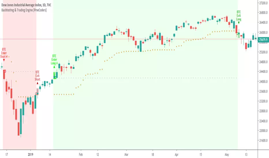
Backtesting & Trading Engine [PineCoders]The PineCoders Backtesting and Trading Engine is a sophisticated framework with hybrid code that can run as a study to generate alerts for automated or discretionary trading while simultaneously providing backtest results. It can also easily be converted to a TradingView strategy in order to run TV backtesting. The Engine comes with many built-in strats for entries, filters, stops and exits, but you can also add you own.
If, like any self-respecting strategy modeler should, you spend a reasonable amount of time constantly researching new strategies and tinkering, our hope is that the Engine will become your inseparable go-to tool to test the validity of your creations, as once your tests are conclusive, you will be able to run this code as a study to generate the alerts required to put it in real-world use, whether for discretionary trading or to interface with an execution bot/app. You may also find the backtesting results the Engine produces in study mode enough for your needs and spend most of your time there, only occasionally converting to strategy mode in order to backtest using TV backtesting.
As you will quickly grasp when you bring up this script’s Settings, this is a complex tool. While you will be able to see results very quickly by just putting it on a chart and using its built-in strategies, in order to reap the full benefits of the PineCoders Engine, you will need to invest the time required to understand the subtleties involved in putting all its potential into play.
Disclaimer: use the Engine at your own risk.
Before we delve in more detail, here’s a bird’s eye view of the Engine’s features:
More than 40 built-in strategies,
Customizable components,
Coupling with your own external indicator,
Simple conversion from Study to Strategy modes,
Post-Exit analysis to search for alternate trade outcomes,
Use of the Data Window to show detailed bar by bar trade information and global statistics, including some not provided by TV backtesting,
Plotting of reminders and generation of alerts on in-trade events.
By combining your own strats to the built-in strats supplied with the Engine, and then tuning the numerous options and parameters in the Inputs dialog box, you will be able to play what-if scenarios from an infinite number of permutations.
USE CASES
You have written an indicator that provides an entry strat but it’s missing other components like a filter and a stop strategy. You add a plot in your indicator that respects the Engine’s External Signal Protocol, connect it to the Engine by simply selecting your indicator’s plot name in the Engine’s Settings/Inputs and then run tests on different combinations of entry stops, in-trade stops and profit taking strats to find out which one produces the best results with your entry strat.
You are building a complex strategy that you will want to run as an indicator generating alerts to be sent to a third-party execution bot. You insert your code in the Engine’s modules and leverage its trade management code to quickly move your strategy into production.
You have many different filters and want to explore results using them separately or in combination. Integrate the filter code in the Engine and run through different permutations or hook up your filtering through the external input and control your filter combos from your indicator.
You are tweaking the parameters of your entry, filter or stop strat. You integrate it in the Engine and evaluate its performance using the Engine’s statistics.
You always wondered what results a random entry strat would yield on your markets. You use the Engine’s built-in random entry strat and test it using different combinations of filters, stop and exit strats.
You want to evaluate the impact of fees and slippage on your strategy. You use the Engine’s inputs to play with different values and get immediate feedback in the detailed numbers provided in the Data Window.
You just want to inspect the individual trades your strategy generates. You include it in the Engine and then inspect trades visually on your charts, looking at the numbers in the Data Window as you move your cursor around.
You have never written a production-grade strategy and you want to learn how. Inspect the code in the Engine; you will find essential components typical of what is being used in actual trading systems.
You have run your system for a while and have compiled actual slippage information and your broker/exchange has updated his fees schedule. You enter the information in the Engine and run it on your markets to see the impact this has on your results.
FEATURES
Before going into the detail of the Inputs and the Data Window numbers, here’s a more detailed overview of the Engine’s features.
Built-in strats
The engine comes with more than 40 pre-coded strategies for the following standard system components:
Entries,
Filters,
Entry stops,
2 stage in-trade stops with kick-in rules,
Pyramiding rules,
Hard exits.
While some of the filter and stop strats provided may be useful in production-quality systems, you will not devise crazy profit-generating systems using only the entry strats supplied; that part is still up to you, as will be finding the elusive combination of components that makes winning systems. The Engine will, however, provide you with a solid foundation where all the trade management nitty-gritty is handled for you. By binding your custom strats to the Engine, you will be able to build reliable systems of the best quality currently allowed on the TV platform.
On-chart trade information
As you move over the bars in a trade, you will see trade numbers in the Data Window change at each bar. The engine calculates the P&L at every bar, including slippage and fees that would be incurred were the trade exited at that bar’s close. If the trade includes pyramided entries, those will be taken into account as well, although for those, final fees and slippage are only calculated at the trade’s exit.
You can also see on-chart markers for the entry level, stop positions, in-trade special events and entries/exits (you will want to disable these when using the Engine in strategy mode to see TV backtesting results).
Customization
You can couple your own strats to the Engine in two ways:
1. By inserting your own code in the Engine’s different modules. The modular design should enable you to do so with minimal effort by following the instructions in the code.
2. By linking an external indicator to the engine. After making the proper selections in the engine’s Settings and providing values respecting the engine’s protocol, your external indicator can, when the Engine is used in Indicator mode only:
Tell the engine when to enter long or short trades, but let the engine’s in-trade stop and exit strats manage the exits,
Signal both entries and exits,
Provide an entry stop along with your entry signal,
Filter other entry signals generated by any of the engine’s entry strats.
Conversion from strategy to study
TradingView strategies are required to backtest using the TradingView backtesting feature, but if you want to generate alerts with your script, whether for automated trading or just to trigger alerts that you will use in discretionary trading, your code has to run as a study since, for the time being, strategies can’t generate alerts. From hereon we will use indicator as a synonym for study.
Unless you want to maintain two code bases, you will need hybrid code that easily flips between strategy and indicator modes, and your code will need to restrict its use of strategy() calls and their arguments if it’s going to be able to run both as an indicator and a strategy using the same trade logic. That’s one of the benefits of using this Engine. Once you will have entered your own strats in the Engine, it will be a matter of commenting/uncommenting only four lines of code to flip between indicator and strategy modes in a matter of seconds.
Additionally, even when running in Indicator mode, the Engine will still provide you with precious numbers on your individual trades and global results, some of which are not available with normal TradingView backtesting.
Post-Exit Analysis for alternate outcomes (PEA)
While typical backtesting shows results of trade outcomes, PEA focuses on what could have happened after the exit. The intention is to help traders get an idea of the opportunity/risk in the bars following the trade in order to evaluate if their exit strategies are too aggressive or conservative.
After a trade is exited, the Engine’s PEA module continues analyzing outcomes for a user-defined quantity of bars. It identifies the maximum opportunity and risk available in that space, and calculates the drawdown required to reach the highest opportunity level post-exit, while recording the number of bars to that point.
Typically, if you can’t find opportunity greater than 1X past your trade using a few different reasonable lengths of PEA, your strategy is doing pretty good at capturing opportunity. Remember that 100% of opportunity is never capturable. If, however, PEA was finding post-trade maximum opportunity of 3 or 4X with average drawdowns of 0.3 to those areas, this could be a clue revealing your system is exiting trades prematurely. To analyze PEA numbers, you can uncomment complete sets of plots in the Plot module to reveal detailed global and individual PEA numbers.
Statistics
The Engine provides stats on your trades that TV backtesting does not provide, such as:
Average Profitability Per Trade (APPT), aka statistical expectancy, a crucial value.
APPT per bar,
Average stop size,
Traded volume .
It also shows you on a trade-by-trade basis, on-going individual trade results and data.
In-trade events
In-trade events can plot reminders and trigger alerts when they occur. The built-in events are:
Price approaching stop,
Possible tops/bottoms,
Large stop movement (for discretionary trading where stop is moved manually),
Large price movements.
Slippage and Fees
Even when running in indicator mode, the Engine allows for slippage and fees to be included in the logic and test results.
Alerts
The alert creation mechanism allows you to configure alerts on any combination of the normal or pyramided entries, exits and in-trade events.
Backtesting results
A few words on the numbers calculated in the Engine. Priority is given to numbers not shown in TV backtesting, as you can readily convert the script to a strategy if you need them.
We have chosen to focus on numbers expressing results relative to X (the trade’s risk) rather than in absolute currency numbers or in other more conventional but less useful ways. For example, most of the individual trade results are not shown in percentages, as this unit of measure is often less meaningful than those expressed in units of risk (X). A trade that closes with a +25% result, for example, is a poor outcome if it was entered with a -50% stop. Expressed in X, this trade’s P&L becomes 0.5, which provides much better insight into the trade’s outcome. A trade that closes with a P&L of +2X has earned twice the risk incurred upon entry, which would represent a pre-trade risk:reward ratio of 2.
The way to go about it when you think in X’s and that you adopt the sound risk management policy to risk a fixed percentage of your account on each trade is to equate a currency value to a unit of X. E.g. your account is 10K USD and you decide you will risk a maximum of 1% of it on each trade. That means your unit of X for each trade is worth 100 USD. If your APPT is 2X, this means every time you risk 100 USD in a trade, you can expect to make, on average, 200 USD.
By presenting results this way, we hope that the Engine’s statistics will appeal to those cognisant of sound risk management strategies, while gently leading traders who aren’t, towards them.
We trade to turn in tangible profits of course, so at some point currency must come into play. Accordingly, some values such as equity, P&L, slippage and fees are expressed in currency.
Many of the usual numbers shown in TV backtests are nonetheless available, but they have been commented out in the Engine’s Plot module.
Position sizing and risk management
All good system designers understand that optimal risk management is at the very heart of all winning strategies. The risk in a trade is defined by the fraction of current equity represented by the amplitude of the stop, so in order to manage risk optimally on each trade, position size should adjust to the stop’s amplitude. Systems that enter trades with a fixed stop amplitude can get away with calculating position size as a fixed percentage of current equity. In the context of a test run where equity varies, what represents a fixed amount of risk translates into different currency values.
Dynamically adjusting position size throughout a system’s life is optimal in many ways. First, as position sizing will vary with current equity, it reproduces a behavioral pattern common to experienced traders, who will dial down risk when confronted to poor performance and increase it when performance improves. Second, limiting risk confers more predictability to statistical test results. Third, position sizing isn’t just about managing risk, it’s also about maximizing opportunity. By using the maximum leverage (no reference to trading on margin here) into the trade that your risk management strategy allows, a dynamic position size allows you to capture maximal opportunity.
To calculate position sizes using the fixed risk method, we use the following formula: Position = Account * MaxRisk% / Stop% [, which calculates a position size taking into account the trade’s entry stop so that if the trade is stopped out, 100 USD will be lost. For someone who manages risk this way, common instructions to invest a certain percentage of your account in a position are simply worthless, as they do not take into account the risk incurred in the trade.
The Engine lets you select either the fixed risk or fixed percentage of equity position sizing methods. The closest thing to dynamic position sizing that can currently be done with alerts is to use a bot that allows syntax to specify position size as a percentage of equity which, while being dynamic in the sense that it will adapt to current equity when the trade is entered, does not allow us to modulate position size using the stop’s amplitude. Changes to alerts are on the way which should solve this problem.
In order for you to simulate performance with the constraint of fixed position sizing, the Engine also offers a third, less preferable option, where position size is defined as a fixed percentage of initial capital so that it is constant throughout the test and will thus represent a varying proportion of current equity.
Let’s recap. The three position sizing methods the Engine offers are:
1. By specifying the maximum percentage of risk to incur on your remaining equity, so the Engine will dynamically adjust position size for each trade so that, combining the stop’s amplitude with position size will yield a fixed percentage of risk incurred on current equity,
2. By specifying a fixed percentage of remaining equity. Note that unless your system has a fixed stop at entry, this method will not provide maximal risk control, as risk will vary with the amplitude of the stop for every trade. This method, as the first, does however have the advantage of automatically adjusting position size to equity. It is the Engine’s default method because it has an equivalent in TV backtesting, so when flipping between indicator and strategy mode, test results will more or less correspond.
3. By specifying a fixed percentage of the Initial Capital. While this is the least preferable method, it nonetheless reflects the reality confronted by most system designers on TradingView today. In this case, risk varies both because the fixed position size in initial capital currency represents a varying percentage of remaining equity, and because the trade’s stop amplitude may vary, adding another variability vector to risk.
Note that the Engine cannot display equity results for strategies entering trades for a fixed amount of shares/contracts at a variable price.
SETTINGS/INPUTS
Because the initial text first published with a script cannot be edited later and because there are just too many options, the Engine’s Inputs will not be covered in minute detail, as they will most certainly evolve. We will go over them with broad strokes; you should be able to figure the rest out. If you have questions, just ask them here or in the PineCoders Telegram group.
Display
The display header’s checkbox does nothing.
For the moment, only one exit strategy uses a take profit level, so only that one will show information when checking “Show Take Profit Level”.
Entries
You can activate two simultaneous entry strats, each selected from the same set of strats contained in the Engine. If you select two and they fire simultaneously, the main strat’s signal will be used.
The random strat in each list uses a different seed, so you will get different results from each.
The “Filter transitions” and “Filter states” strats delegate signal generation to the selected filter(s). “Filter transitions” signals will only fire when the filter transitions into bull/bear state, so after a trade is stopped out, the next entry may take some time to trigger if the filter’s state does not change quickly. When you choose “Filter states”, then a new trade will be entered immediately after an exit in the direction the filter allows.
If you select “External Indicator”, your indicator will need to generate a +2/-2 (or a positive/negative stop value) to enter a long/short position, providing the selected filters allow for it. If you wish to use the Engine’s capacity to also derive the entry stop level from your indicator’s signal, then you must explicitly choose this option in the Entry Stops section.
Filters
You can activate as many filters as you wish; they are additive. The “Maximum stop allowed on entry” is an important component of proper risk management. If your system has an average 3% stop size and you need to trade using fixed position sizes because of alert/execution bot limitations, you must use this filter because if your system was to enter a trade with a 15% stop, that trade would incur 5 times the normal risk, and its result would account for an abnormally high proportion in your system’s performance.
Remember that any filter can also be used as an entry signal, either when it changes states, or whenever no trade is active and the filter is in a bull or bear mode.
Entry Stops
An entry stop must be selected in the Engine, as it requires a stop level before the in-trade stop is calculated. Until the selected in-trade stop strat generates a stop that comes closer to price than the entry stop (or respects another one of the in-trade stops kick in strats), the entry stop level is used.
It is here that you must select “External Indicator” if your indicator supplies a +price/-price value to be used as the entry stop. A +price is expected for a long entry and a -price value will enter a short with a stop at price. Note that the price is the absolute price, not an offset to the current price level.
In-Trade Stops
The Engine comes with many built-in in-trade stop strats. Note that some of them share the “Length” and “Multiple” field, so when you swap between them, be sure that the length and multiple in use correspond to what you want for that stop strat. Suggested defaults appear with the name of each strat in the dropdown.
In addition to the strat you wish to use, you must also determine when it kicks in to replace the initial entry’s stop, which is determined using different strats. For strats where you can define a positive or negative multiple of X, percentage or fixed value for a kick-in strat, a positive value is above the trade’s entry fill and a negative one below. A value of zero represents breakeven.
Pyramiding
What you specify in this section are the rules that allow pyramiding to happen. By themselves, these rules will not generate pyramiding entries. For those to happen, entry signals must be issued by one of the active entry strats, and conform to the pyramiding rules which act as a filter for them. The “Filter must allow entry” selection must be chosen if you want the usual system’s filters to act as additional filtering criteria for your pyramided entries.
Hard Exits
You can choose from a variety of hard exit strats. Hard exits are exit strategies which signal trade exits on specific events, as opposed to price breaching a stop level in In-Trade Stops strategies. They are self-explanatory. The last one labelled When Take Profit Level (multiple of X) is reached is the only one that uses a level, but contrary to stops, it is above price and while it is relative because it is expressed as a multiple of X, it does not move during the trade. This is the level called Take Profit that is show when the “Show Take Profit Level” checkbox is checked in the Display section.
While stops focus on managing risk, hard exit strategies try to put the emphasis on capturing opportunity.
Slippage
You can define it as a percentage or a fixed value, with different settings for entries and exits. The entry and exit markers on the chart show the impact of slippage on the entry price (the fill).
Fees
Fees, whether expressed as a percentage of position size in and out of the trade or as a fixed value per in and out, are in the same units of currency as the capital defined in the Position Sizing section. Fees being deducted from your Capital, they do not have an impact on the chart marker positions.
In-Trade Events
These events will only trigger during trades. They can be helpful to act as reminders for traders using the Engine as assistance to discretionary trading.
Post-Exit Analysis
It is normally on. Some of its results will show in the Global Numbers section of the Data Window. Only a few of the statistics generated are shown; many more are available, but commented out in the Plot module.
Date Range Filtering
Note that you don’t have to change the dates to enable/diable filtering. When you are done with a specific date range, just uncheck “Date Range Filtering” to disable date filtering.
Alert Triggers
Each selection corresponds to one condition. Conditions can be combined into a single alert as you please. Just be sure you have selected the ones you want to trigger the alert before you create the alert. For example, if you trade in both directions and you want a single alert to trigger on both types of exits, you must select both “Long Exit” and “Short Exit” before creating your alert.
Once the alert is triggered, these settings no longer have relevance as they have been saved with the alert.
When viewing charts where an alert has just triggered, if your alert triggers on more than one condition, you will need the appropriate markers active on your chart to figure out which condition triggered the alert, since plotting of markers is independent of alert management.
Position sizing
You have 3 options to determine position size:
1. Proportional to Stop -> Variable, with a cap on size.
2. Percentage of equity -> Variable.
3. Percentage of Initial Capital -> Fixed.
External Indicator
This is where you connect your indicator’s plot that will generate the signals the Engine will act upon. Remember this only works in Indicator mode.
DATA WINDOW INFORMATION
The top part of the window contains global numbers while the individual trade information appears in the bottom part. The different types of units used to express values are:
curr: denotes the currency used in the Position Sizing section of Inputs for the Initial Capital value.
quote: denotes quote currency, i.e. the value the instrument is expressed in, or the right side of the market pair (USD in EURUSD ).
X: the stop’s amplitude, itself expressed in quote currency, which we use to express a trade’s P&L, so that a trade with P&L=2X has made twice the stop’s amplitude in profit. This is sometimes referred to as R, since it represents one unit of risk. It is also the unit of measure used in the APPT, which denotes expected reward per unit of risk.
X%: is also the stop’s amplitude, but expressed as a percentage of the Entry Fill.
The numbers appearing in the Data Window are all prefixed:
“ALL:” the number is the average for all first entries and pyramided entries.
”1ST:” the number is for first entries only.
”PYR:” the number is for pyramided entries only.
”PEA:” the number is for Post-Exit Analyses
Global Numbers
Numbers in this section represent the results of all trades up to the cursor on the chart.
Average Profitability Per Trade (X): This value is the most important gauge of your strat’s worthiness. It represents the returns that can be expected from your strat for each unit of risk incurred. E.g.: your APPT is 2.0, thus for every unit of currency you invest in a trade, you can on average expect to obtain 2 after the trade. APPT is also referred to as “statistical expectancy”. If it is negative, your strategy is losing, even if your win rate is very good (it means your winning trades aren’t winning enough, or your losing trades lose too much, or both). Its counterpart in currency is also shown, as is the APPT/bar, which can be a useful gauge in deciding between rivalling systems.
Profit Factor: Gross of winning trades/Gross of losing trades. Strategy is profitable when >1. Not as useful as the APPT because it doesn’t take into account the win rate and the average win/loss per trade. It is calculated from the total winning/losing results of this particular backtest and has less predictive value than the APPT. A good profit factor together with a poor APPT means you just found a chart where your system outperformed. Relying too much on the profit factor is a bit like a poker player who would think going all in with two’s against aces is optimal because he just won a hand that way.
Win Rate: Percentage of winning trades out of all trades. Taken alone, it doesn’t have much to do with strategy profitability. You can have a win rate of 99% but if that one trade in 100 ruins you because of poor risk management, 99% doesn’t look so good anymore. This number speaks more of the system’s profile than its worthiness. Still, it can be useful to gauge if the system fits your personality. It can also be useful to traders intending to sell their systems, as low win rate systems are more difficult to sell and require more handholding of worried customers.
Equity (curr): This the sum of initial capital and the P&L of your system’s trades, including fees and slippage.
Return on Capital is the equivalent of TV’s Net Profit figure, i.e. the variation on your initial capital.
Maximum drawdown is the maximal drawdown from the highest equity point until the drop . There is also a close to close (meaning it doesn’t take into account in-trade variations) maximum drawdown value commented out in the code.
The next values are self-explanatory, until:
PYR: Avg Profitability Per Entry (X): this is the APPT for all pyramided entries.
PEA: Avg Max Opp . Available (X): the average maximal opportunity found in the Post-Exit Analyses.
PEA: Avg Drawdown to Max Opp . (X): this represents the maximum drawdown (incurred from the close at the beginning of the PEA analysis) required to reach the maximal opportunity point.
Trade Information
Numbers in this section concern only the current trade under the cursor. Most of them are self-explanatory. Use the description’s prefix to determine what the values applies to.
PYR: Avg Profitability Per Entry (X): While this value includes the impact of all current pyramided entries (and only those) and updates when you move your cursor around, P&L only reflects fees at the trade’s last bar.
PEA: Max Opp . Available (X): It’s the most profitable close reached post-trade, measured from the trade’s Exit Fill, expressed in the X value of the trade the PEA follows.
PEA: Drawdown to Max Opp . (X): This is the maximum drawdown from the trade’s Exit Fill that needs to be sustained in order to reach the maximum opportunity point, also expressed in X. Note that PEA numbers do not include slippage and fees.
EXTERNAL SIGNAL PROTOCOL
Only one external indicator can be connected to a script; in order to leverage its use to the fullest, the engine provides options to use it as either an entry signal, an entry/exit signal or a filter. When used as an entry signal, you can also use the signal to provide the entry’s stop. Here’s how this works:
For filter state: supply +1 for bull (long entries allowed), -1 for bear (short entries allowed).
For entry signals: supply +2 for long, -2 for short.
For exit signals: supply +3 for exit from long, -3 for exit from short.
To send an entry stop level with an entry signal: Send positive stop level for long entry (e.g. 103.33 to enter a long with a stop at 103.33), negative stop level for short entry (e.g. -103.33 to enter a short with a stop at 103.33). If you use this feature, your indicator will have to check for exact stop levels of 1.0, 2.0 or 3.0 and their negative counterparts, and fudge them with a tick in order to avoid confusion with other signals in the protocol.
Remember that mere generation of the values by your indicator will have no effect until you explicitly allow their use in the appropriate sections of the Engine’s Settings/Inputs.
An example of a script issuing a signal for the Engine is published by PineCoders.
RECOMMENDATIONS TO ASPIRING SYSTEM DESIGNERS
Stick to higher timeframes. On progressively lower timeframes, margins decrease and fees and slippage take a proportionally larger portion of profits, to the point where they can very easily turn a profitable strategy into a losing one. Additionally, your margin for error shrinks as the equilibrium of your system’s profitability becomes more fragile with the tight numbers involved in the shorter time frames. Avoid <1H time frames.
Know and calculate fees and slippage. To avoid market shock, backtest using conservative fees and slippage parameters. Systems rarely show unexpectedly good returns when they are confronted to the markets, so put all chances on your side by being outrageously conservative—or a the very least, realistic. Test results that do not include fees and slippage are worthless. Slippage is there for a reason, and that’s because our interventions in the market change the market. It is easier to find alpha in illiquid markets such as cryptos because not many large players participate in them. If your backtesting results are based on moving large positions and you don’t also add the inevitable slippage that will occur when you enter/exit thin markets, your backtesting will produce unrealistic results. Even if you do include large slippage in your settings, the Engine can only do so much as it will not let slippage push fills past the high or low of the entry bar, but the gap may be much larger in illiquid markets.
Never test and optimize your system on the same dataset , as that is the perfect recipe for overfitting or data dredging, which is trying to find one precise set of rules/parameters that works only on one dataset. These setups are the most fragile and often get destroyed when they meet the real world.
Try to find datasets yielding more than 100 trades. Less than that and results are not as reliable.
Consider all backtesting results with suspicion. If you never entertained sceptic tendencies, now is the time to begin. If your backtest results look really good, assume they are flawed, either because of your methodology, the data you’re using or the software doing the testing. Always assume the worse and learn proper backtesting techniques such as monte carlo simulations and walk forward analysis to avoid the traps and biases that unchecked greed will set for you. If you are not familiar with concepts such as survivor bias, lookahead bias and confirmation bias, learn about them.
Stick to simple bars or candles when designing systems. Other types of bars often do not yield reliable results, whether by design (Heikin Ashi) or because of the way they are implemented on TV (Renko bars).
Know that you don’t know and use that knowledge to learn more about systems and how to properly test them, about your biases, and about yourself.
Manage risk first , then capture opportunity.
Respect the inherent uncertainty of the future. Cleanse yourself of the sad arrogance and unchecked greed common to newcomers to trading. Strive for rationality. Respect the fact that while backtest results may look promising, there is no guarantee they will repeat in the future (there is actually a high probability they won’t!), because the future is fundamentally unknowable. If you develop a system that looks promising, don’t oversell it to others whose greed may lead them to entertain unreasonable expectations.
Have a plan. Understand what king of trading system you are trying to build. Have a clear picture or where entries, exits and other important levels will be in the sort of trade you are trying to create with your system. This stated direction will help you discard more efficiently many of the inevitably useless ideas that will pop up during system design.
Be wary of complexity. Experienced systems engineers understand how rapidly complexity builds when you assemble components together—however simple each one may be. The more complex your system, the more difficult it will be to manage.
Play! . Allow yourself time to play around when you design your systems. While much comes about from working with a purpose, great ideas sometimes come out of just trying things with no set goal, when you are stuck and don’t know how to move ahead. Have fun!
@LucF
NOTES
While the engine’s code can supply multiple consecutive entries of longs or shorts in order to scale positions (pyramid), all exits currently assume the execution bot will exit the totality of the position. No partial exits are currently possible with the Engine.
Because the Engine is literally crippled by the limitations on the number of plots a script can output on TV; it can only show a fraction of all the information it calculates in the Data Window. You will find in the Plot Module vast amounts of commented out lines that you can activate if you also disable an equivalent number of other plots. This may be useful to explore certain characteristics of your system in more detail.
When backtesting using the TV backtesting feature, you will need to provide the strategy parameters you wish to use through either Settings/Properties or by changing the default values in the code’s header. These values are defined in variables and used not only in the strategy() statement, but also as defaults in the Engine’s relevant Inputs.
If you want to test using pyramiding, then both the strategy’s Setting/Properties and the Engine’s Settings/Inputs need to allow pyramiding.
If you find any bugs in the Engine, please let us know.
THANKS
To @glaz for allowing the use of his unpublished MA Squize in the filters.
To @everget for his Chandelier stop code, which is also used as a filter in the Engine.
To @RicardoSantos for his pseudo-random generator, and because it’s from him that I first read in the Pine chat about the idea of using an external indicator as input into another. In the PineCoders group, @theheirophant then mentioned the idea of using it as a buy/sell signal and @simpelyfe showed a piece of code implementing the idea. That’s the tortuous story behind the use of the external indicator in the Engine.
To @admin for the Volatility stop’s original code and for the donchian function lifted from Ichimoku .
To @BobHoward21 for the v3 version of Volatility Stop .
To @scarf and @midtownsk8rguy for the color tuning.
To many other scripters who provided encouragement and suggestions for improvement during the long process of writing and testing this piece of code.
To J. Welles Wilder Jr. for ATR, used extensively throughout the Engine.
To TradingView for graciously making an account available to PineCoders.
And finally, to all fellow PineCoders for the constant intellectual stimulation; it is a privilege to share ideas with you all. The Engine is for all TradingView PineCoders, of course—but especially for you.
Look first. Then leap.
Great Expectations [LucF]Great Expectations helps traders answer the question: What is possible? It is a powerful question, yet exploration of the unknown always entails risk. A more complete set of questions better suited to traders could be:
What opportunity exists from any given point on a chart?
What portion of this opportunity can be realistically captured?
What risk will be incurred in trying to do so, and how long will it take?
Great Expectations is the result of an exploration of these questions. It is a trade simulator that generates visual and quantitative information to help strategy modelers visually identify and analyse areas of optimal expectation on charts, whether they are designing automated or discretionary strategies.
WARNING: Great Expectations is NOT an indicator that helps determine the current state of a market. It works by looking at points in the past from which the future is already known. It uses one definition of repainting extensively (i.e. it goes back in the past to print information that could not have been know at the time). Repainting understood that way is in fact almost all the indicator does! —albeit for what I hope is a noble cause. The indicator is of no use whatsoever in analyzing markets in real-time. If you do not understand what it does, please stay away!
This is an indicator—not a strategy that uses TradingView’s backtesting engine. It works by simulating trades, not unlike a backtest, but with the crucial difference that it assumes a trade (either long or short) is entered on all bars in the historic sample. It walks forward from each bar and determines possible outcomes, gathering individual trade statistics that in turn generate precious global statistics from all outcomes tested on the chart.
Great Expectations provides numbers summarizing trade results on all simulations run from the chart. Those numbers cannot be compared to backtest-produced numbers since all non-filtered bars are examined, even if an entry was taken on the bar immediately preceding the current one, which never happens in a backtest. This peculiarity does NOT invalidate Great Expectations calculations; it just entails that results be considered under a different light. Provided they are evaluated within the indicator’s context, they can be useful—sometimes even more than backtesting results, e.g. in evaluating the impact of parameter-fitting or variations in entry, exit or filtering strats.
Traders and strategy modelers are creatures of hope often suffering from blurred vision; my hope is that Great Expectations will help them appraise the validity of their setup and strat intuitions in a realistic fashion, preventing confirmation bias from obstructing perspective—and great expectations from turning into financial great deceptions.
USE CASES
You’ve identified what looks like a promising setup on other indicators. You load Great Expectations on the chart and evaluate if its high-expectation areas match locations where your setup’s conditions occur. Unless today is your lucky day, chances are the indicator will help you realize your setup is not as promising as you had hoped.
You want to get a rough estimate of the optimal trade duration for a chart and you don’t mind using the entry and exit strategies provided with the indicator. You use the trade length readouts of the indicator.
You’re experimenting with a new stop strategy and want to know how long it will keep you in trades, on average. You integrate your stop strategy in the indicator’s code and look at the average trade length it produces and the TST ratio to evaluate its performance.
You have put together your own entry and exit criteria and are looking for a filter that will help you improve backtesting results. You visually ascertain the suitability of your filter by looking at its results on the charts with great Expectations, to see if your filter is choosing its areas correctly.
You have a strategy that shows backtested trades on your chart. Great Expectations can help you evaluate how well your strategy is benefitting from high-opportunity areas while avoiding poor expectation spots.
You want more complete statistics on your set of strategies than what backtesting will provide. You use Great Expectations, knowing that it tests all bars in the sample that correspond to your criteria, as opposed to backtesting results which are limited to a subset of all possible entries.
You want to fool your friends into thinking you’ve designed the holy grail of indicators, something that identifies optimal opportunities on any chart; you show them the P&L cloud.
FEATURES
For one trade
At any given point on the chart, assuming a trade is entered there, Great Expectations shows you information specific to that trade simulation both on the chart and in the Data Window.
The chart can display:
the P & L Cloud which shows whether the trade ended profitably or not, and by how much,
the Opportunity & Risk Cloud which the maximum opportunity and risk the simulation encountered. When superimposed over the P & L cloud, you will see what I call the managed opportunity and risk, i.e the portion of maximum opportunity that was captured and the portion of the maximum risk that was incurred,
the target and if it was reached,
a background that uses a gradient to show different levels of trade length, P&L or how frequently the target was reached during simulation.
The Data Window displays more than 40 values on individual trades and global results. For any given trade you will know:
Entry/Exit levels, including slippage impact,
It’s outcome and duration,
P/L achieved,
The fraction of the maximum opportunity/risk managed by the trade.
For all trades
After going through all the possible trades on the chart, the indicator will provide you with a rare view of all outcomes expressed with the P&L cloud, which allows us to instantly see the most/least profitable areas of a chart using trade data as support, while also showing its relationship with the opportunity/risk encountered during the simulation. The difference between the two clouds is the managed opportunity and risk.
The Data Window will present you with numbers which we will go through later. Some of them are: average stop size, P/L, win rate, % opportunity managed, trade lengths for different types of trade outcomes and the TST (Target:Stop Travel) ratio.
Let’s see Great Expectations in action… and remember to open your Data Window!
INPUTS
Trade direction : You must first choose if you wish to look at long or short trades. Because of the way the indicator works and the amount of visual information on the chart, it is only practical to look at one type of trades at a time. The default is Longs.
Maximum trade Length (MaxL) : This is the maximum walk forward distance the simulator will go in analyzing outcomes from any given point in the past. It also determines the size of the dead zone among the chart’s last bars. A red background line identifies the beginning of the dead zone for which not enough bars have elapsed to analyze outcomes for the maximum trade length defined. If an ATR-based entry stop is used, that length is added to the wait time before beginning simulations, so that the first entry starts with a clean ATR value. On a sample of around 16000 bars, my tests show that the indicator runs into server errors at lengths of around 290, i.e. having completed ~4,6M simulation loop iterations. That is way too high a length anyways; 100 will usually be amply enough to ring out all the possibilities out of a simulation, and on shorter time frames, 30 can be enough. While making it unduly small will prevent simulations of expressing the market’s potential, the less you use, the faster the indicator will run. The default is 40.
Unrealized P&L base at End of Trade (EOT) : When a simulation ends and the trade is still open, we calculate unrealized P&L from an exit order executed from either the last in-trade stop on the previous bar, or the close of the last bar. You can readily see the impact of this selection on the chart, with the P&L cloud. The default is on the close.
Display : The check box besides the title does nothing.
Show target : Shows a green line displaying the trade’s target expressed as a multiple of X, i.e. the amplitude of the entry stop. I call this value “X” and use it as a unit to express profit and loss on a trade (some call it “R”). The line is highlighted for trades where the close reached the target during the trade, whether the trade ended in profit or loss. This is also where you specify the multiple of X you wish to use in calculating targets. The multiple is used even if targets are not displayed.
Show P&L Cloud : The cloud allows traders to see right away the profitable areas of the chart. The only line printed with the cloud is the “end of trade line” (EOT). The EOT line is the only way one can see the level where a trade ended on the chart (in the Data Window you can see it as the “Exit Fill” value). The EOT level for the trade determines if the trade ended in a profit or a loss. Its value represents one of the following:
- fill from order executed at close of bar where stop is breached during trade (which produces “Realized P/L”),
- simulation of a fill pseudo-fill at the user-defined EOT level (last close or stop level) if the trade runs its course through MaxL bars without getting stopped (producing Unrealized P/L).
The EOT line and the cloud fill print in green when the trade’s outcome is profitable and in red when it is not. If the trade was closed after breaching the stop, the line appears brighter.
Show Opportunity&Risk Cloud : Displays the maximum opportunity/risk that was present during the trade, i.e. the maximum and minimum prices reached.
Background Color Scheme : Allows you to choose between 3 different color schemes for the background gradients, to accommodate different types of chart background/candles. Select “None” if you don’t want a background.
Background source : Determines what value will be used to generate the different intensities of the gradient. You can choose trade length (brighter is shorter), Trade P&L (brighter is higher) or the number of times the target was reached during simulation (brighter is higher). The default is Trade Length.
Entry strat : The check box besides the title does nothing. The default strat is All bars, meaning a trade will be simulated from all bars not excluded by the filters where a MaxL bars future exists. For fun, I’ve included a pseudo-random entry strat (an indirect way of changing the seed is to vary the starting date of the simulation).
Show Filter State : Displays areas where the combination of filters you have selected are allowing entries. Filtering occurs as per your selection(s), whether the state is displayed or not. The effect of multiple selections is additive. The filters are:
1. Bar direction: Longs will only be entered if close>open and vice versa.
2. Rising Volume: Applies to both long and shorts.
3. Rising/falling MA of the length you choose over the number of bars you choose.
4. Custom indicator: You can feed your own filtering signal through this from another indicator. It must produce a signal of 1 to allow long entries and 0 to allow shorts.
Show Entry Stops :
1. Multiple of user-defined length ATR.
2. Fixed percentage.
3. Fixed value.
All entry stops are calculated using the entry fill price as a reference. The fill price is calculated from the current bar’s open, to which slippage is added if configured. This simulates the case where the strategy issued the entry signal on the previous bar for it to be executed at the next bar’s open.
The entry stop remains active until the in-trade stop becomes the more aggressive of the two stops. From then on, the entry stop will be ignored, unless a bar close breaches the in-trade stop, in which case the stop will be reset with a new entry stop and the process repeats.
Show In-trade stops : Displays in bright red the selected in-trade stop (be sure to read the note in this section about them).
1. ATR multiple: added/subtracted from the average of the two previous bars minimum/maximum of open/close.
2. A trailing stop with a deviation expressed as a multiple of entry stop (X).
3. A fixed percentage trailing stop.
Trailing stops deviations are measured from the highest/lowest high/low reached during the trade.
Note: There is a twist with the in-trade stops. It’s that for any given bar, its in-trade stop can hold multiple values, as each successive pass of the advancing simulation loops goes over it from a different entry points. What is printed is the stop from the loop that ended on that bar, which may have nothing to do with other instances of the trade’s in-trade stop for the same bar when visited from other starting points in previous simulations. There is just no practical way to print all stop values that were used for any given bar. While the printed entry stops are the actual ones used on each bar, the in-trade stops shown are merely the last instance used among many.
Include Slippage : if checked, slippage will be added/subtracted from order price to yield the fill price. Slippage is in percentage. If you choose to include slippage in the simulations, remember to adjust it by considering the liquidity of the markets and the time frame you’ll be analyzing.
Include Fees : if checked, fees will be subtracted/added to both realized an unrealized trade profits/losses. Fees are in percentage. The default fees work well for crypto markets but will need adjusting for others—especially in Forex. Remember to modify them accordingly as they can have a major impact on results. Both fees and slippage are included to remind us of their importance, even if the global numbers produced by the indicator are not representative of a real trading scenario composed of sequential trades.
Date Range filtering : the usual. Just note that the checkbox has to be selected for date filtering to activate.
DATA WINDOW
Most of the information produced by this indicator is made available in the Data Window, which you bring up by using the icon below the Watchlist and Alerts buttons at the right of the TV UI. Here’s what’s there.
Some of the information presented in the Data Window is standard trade data; other values are not so standard; e. g. the notions of managed opportunity and risk and Target:Stop Travel ratio. The interplay between all the values provided by Great Expectations is inherently complex, even for a static set of entry/filter/exit strats. During the constant updating which the habitual process of progressive refinement in building strategies that is the lot of strategy modelers entails, another level of complexity is no doubt added to the analysis of this indicator’s values. While I don’t want to sound like Wolfram presenting A New Kind of Science , I do believe that if you are a serious strategy modeler and spend the time required to get used to using all the information this indicator makes available, you may find it useful.
Trade Information
Entry Order : This is the open of the bar where simulation starts. We suppose that an entry signal was generated at the previous bar.
Entry Fill (including slip.) : The actual entry price, including slippage. This is the base price from which other values will be calculated.
Exit Order : When a stop is breached, an exit order is executed from the close of the bar that breached the stop. While there is no “In-trade stop” value included in the Data Window (other than the End of trade Stop previously discussed), this “Exit Order” value is how we can know the level where the trade was stopped during the simulation. The “Trade Length” value will then show the bar where the stop was breached.
Exit Fill (including slip.) : When the exit order is simulated, slippage is added to the order level to create the fill.
Chart: Target : This is the target calculated at the beginning of the simulation. This value also appear on the chart in teal. It is controlled by the multiple of X defined under the “Show Target” checkbox in the Inputs.
Chart: Entry Stop : This value also appears on the chart (the red dots under points where a trade was simulated). Its value is controlled by the Entry Strat chosen in the Inputs.
X (% Fill, including Fees) and X (currency) : This is the stop’s amplitude (Entry Fill – Entry Stop) + Fees. It represents the risk incurred upon entry and will be used to express P&L. We will show R expressed in both a percentage of the Entry Fill level (this value), and currency (the next value). This value represents the risk in the risk:reward ratio and is considered to be a unit of 1 so that RR can be expressed as a single value (i.e. “2” actually meaning “1:2”).
Trade Length : If trade was stopped, it’s the number of bars elapsed until then. The trade is then considered “Closed”. If the trade ends without being stopped (there is no profit-taking strat implemented, so the stop is the only exit strat), then the trade is “Open”, the length is MaxL and it will show in orange. Otherwise the value will print in green/red to reflect if the trade is winning/losing.
P&L (X) : The P&L of the trade, expressed as a multiple of X, which takes into account fees paid at entry and exit. Given our default target setting at 2 units of “X”, a trade that closes at its target will have produced a P&L of +2.0, i.e. twice the value of X (not counting fees paid at exit ). A trade that gets stopped late 50% further that the entry stop’s level will produce a P&L of -1.5X.
P&L (currency, including Fees) : same value as above, but expressed in currency.
Target first reached at bar : If price closed above the target during the trade (even if it occurs after the trade was stopped), this will show when. This value will be used in calculating our TST ratio.
Times Stop/Target reached in sim. : Includes all occurrences during the complete simulation loop.
Opportunity (X) : The highest/lowest price reached during a simulation, i.e. the maximum opportunity encountered, whether the trade was previously stopped or not, expressed as a multiple of X.
Risk (X) : The lowest/highest price reached during a simulation, i.e. the maximum risk encountered, whether the trade was previously stopped or not, expressed as a multiple of X.
Risk:Opportunity : The greater this ratio, the greater Opportunity is, compared to Risk.
Managed Opportunity (%) : The portion of Opportunity that was captured by the highest/low stop position, even if it occurred after a previous stop closed the trade.
Managed Risk (%) : The portion of risk that was protected by the lowest/highest stop position, even if it occurred after a previous stop closed the trade. When this value is greater than 100%, it means the trade’s stop is protecting more than the maximum risk, which is frequent. You will, however, never see close to those values for the Managed Opportunity value, since the stop would have to be higher than the Maximum opportunity. It is much easier to alleviate the risk than it is to lock in profits.
Managed Risk:Opportunity : The ratio of the two preceding values.
Managed Opp. vs. Risk : The Managed Opportunity minus the Managed Risk. When it is negative, which is most often is, it means your strat is protecting a greater portion of the risk than it captures opportunity.
Global Numbers
Win Rate(%) : Percentage of winning trades over all entries. Open trades are considered winning if their last stop/close (as per user selection) locks in profits.
Avg X%, Avg X (currency) : Averages of previously described values:.
Avg Profitability/Trade (APPT) : This measures expectation using: Average Profitability Per Trade = (Probability of Win × Average Win) − (Probability of Loss × Average Loss) . It quantifies the average expectation/trade, which RR alone can’t do, as the probabilities of each outcome (win/lose) must also be used to calculate expectancy. The APPT combine the RR with the win rate to yield the true expectancy of a strategy. In my usual way of expressing risk with X, APPT is the equivalent of the average P&L per trade expressed in X. An APPT of -1.5 means that we lose on average 1.5X/trade.
Equity (X), Equity (currency) : The cumulative result of all trade outcomes, expressed as a multiple of X. Multiplied by the Average X in currency, this yields the Equity in currency.
Risk:Opportunity, Managed Risk:Opportunity, Managed Opp. vs. Risk : The global values of the ones previously described.
Avg Trade Length (TL) : One of the most important values derived by going through all the simulations. Again, it is composed of either the length of stopped trades, or MaxL when the trade isn’t stopped (open). This value can help systems modelers shape the characteristics of the components they use to build their strategies.
Avg Closed Win TL and Avg Closed Lose TL : The average lengths of winning/losing trades that were stopped.
Target reached? Avg bars to Stop and Target reached? Avg bars to Target : For the trades where the target was reached at some point in the simulation, the number of bars to the first point where the stop was breached and where the target was reached, respectively. These two values are used to calculate the next value.
TST (Target:Stop Travel Ratio) : This tracks the ratio between the two preceding values (Bars to first stop/Bars to first target), but only for trades where the target was reached somewhere in the loop. A ratio of 2 means targets are reached twice as fast as stops.
The next values of this section are counts or percentages and are self-explanatory.
Chart Plots
Contains chart plots of values already describes.
NOTES
Optimization/Overfitting: There is a fine line between optimizing and overfitting. Tools like this indicator can lead unsuspecting modelers down a path of overfitting that often turns strategies into over-specialized beasts that do not perform elegantly when confronted to the real-world. Proven testing strategies like walk forward analysis will go a long way in helping modelers alleviate this risk.
Input tuning: Because the results generated by the indicator will vary with the parameters used in the active entry, filtering and exit strats, it’s important to realize that although it may be fun at first, just slapping the default settings on a chart and time frame will not yield optimal nor reliable results. While using ATR as often as possible (as I do in this indicator) is a good way to make strat parametrization adaptable, it is not a foolproof solution.
There is no data for the last MaxL bars of the chart, since not enough trade future has elapsed to run a simulation from MaxL bars back.
Modifying the code: I have tried to structure the code modularly, even if that entails a larger code base, so that you can adapt it to your needs. I’ve included a few token components in each of the placeholders designed for entry strategies, filters, entry stops and in-trade stops. This will hopefully make it easier to add your own. In the same spirit, I have also commented liberally.
You will find in the code many instances of standard trade management tasks that can be lifted to code TV strategies where, as I do in mine, you manage everything yourself and don’t rely on built-in Pine strategy functions to act on your trades.
Enjoy!
THANKS
To @scarf who showed me how plotchar() could be used to plot values without ruining scale.
To @glaz for the suggestion to include a Chandelier stop strat; I will.
To @simpelyfe for the idea of using an indicator input for the filters (if some day TV lets us use more than one, it will be useful in other modules of the indicator).
To @RicardoSantos for the random generator used in the random entry strat.
To all scripters publishing open source on TradingView; their code is the best way to learn.
To my trading buddies Irving and Bruno; who showed me way back how pro traders get it done.
Adaptive Genesis Engine [AGE]ADAPTIVE GENESIS ENGINE (AGE)
Pure Signal Evolution Through Genetic Algorithms
Where Darwin Meets Technical Analysis
🧬 WHAT YOU'RE GETTING - THE PURE INDICATOR
This is a technical analysis indicator - it generates signals, visualizes probability, and shows you the evolutionary process in real-time. This is NOT a strategy with automatic execution - it's a sophisticated signal generation system that you control .
What This Indicator Does:
Generates Long/Short entry signals with probability scores (35-88% range)
Evolves a population of up to 12 competing strategies using genetic algorithms
Validates strategies through walk-forward optimization (train/test cycles)
Visualizes signal quality through premium gradient clouds and confidence halos
Displays comprehensive metrics via enhanced dashboard
Provides alerts for entries and exits
Works on any timeframe, any instrument, any broker
What This Indicator Does NOT Do:
Execute trades automatically
Manage positions or calculate position sizes
Place orders on your behalf
Make trading decisions for you
This is pure signal intelligence. AGE tells you when and how confident it is. You decide whether and how much to trade.
🔬 THE SCIENCE: GENETIC ALGORITHMS MEET TECHNICAL ANALYSIS
What Makes This Different - The Evolutionary Foundation
Most indicators are static - they use the same parameters forever, regardless of market conditions. AGE is alive . It maintains a population of competing strategies that evolve, adapt, and improve through natural selection principles:
Birth: New strategies spawn through crossover breeding (combining DNA from fit parents) plus random mutation for exploration
Life: Each strategy trades virtually via shadow portfolios, accumulating wins/losses, tracking drawdown, and building performance history
Selection: Strategies are ranked by comprehensive fitness scoring (win rate, expectancy, drawdown control, signal efficiency)
Death: Weak strategies are culled periodically, with elite performers (top 2 by default) protected from removal
Evolution: The gene pool continuously improves as successful traits propagate and unsuccessful ones die out
This is not curve-fitting. Each new strategy must prove itself on out-of-sample data through walk-forward validation before being trusted for live signals.
🧪 THE DNA: WHAT EVOLVES
Every strategy carries a 10-gene chromosome controlling how it interprets market data:
Signal Sensitivity Genes
Entropy Sensitivity (0.5-2.0): Weight given to market order/disorder calculations. Low values = conservative, require strong directional clarity. High values = aggressive, act on weaker order signals.
Momentum Sensitivity (0.5-2.0): Weight given to RSI/ROC/MACD composite. Controls responsiveness to momentum shifts vs. mean-reversion setups.
Structure Sensitivity (0.5-2.0): Weight given to support/resistance positioning. Determines how much price location within swing range matters.
Probability Adjustment Genes
Probability Boost (-0.10 to +0.10): Inherent bias toward aggressive (+) or conservative (-) entries. Acts as personality trait - some strategies naturally optimistic, others pessimistic.
Trend Strength Requirement (0.3-0.8): Minimum trend conviction needed before signaling. Higher values = only trades strong trends, lower values = acts in weak/sideways markets.
Volume Filter (0.5-1.5): Strictness of volume confirmation. Higher values = requires strong volume, lower values = volume less important.
Risk Management Genes
ATR Multiplier (1.5-4.0): Base volatility scaling for all price levels. Controls whether strategy uses tight or wide stops/targets relative to ATR.
Stop Multiplier (1.0-2.5): Stop loss tightness. Lower values = aggressive profit protection, higher values = more breathing room.
Target Multiplier (1.5-4.0): Profit target ambition. Lower values = quick scalping exits, higher values = swing trading holds.
Adaptation Gene
Regime Adaptation (0.0-1.0): How much strategy adjusts behavior based on detected market regime (trending/volatile/choppy). Higher values = more reactive to regime changes.
The Magic: AGE doesn't just try random combinations. Through tournament selection and fitness-weighted crossover, successful gene combinations spread through the population while unsuccessful ones fade away. Over 50-100 bars, you'll see the population converge toward genes that work for YOUR instrument and timeframe.
📊 THE SIGNAL ENGINE: THREE-LAYER SYNTHESIS
Before any strategy generates a signal, AGE calculates probability through multi-indicator confluence:
Layer 1 - Market Entropy (Information Theory)
Measures whether price movements exhibit directional order or random walk characteristics:
The Math:
Shannon Entropy = -Σ(p × log(p))
Market Order = 1 - (Entropy / 0.693)
What It Means:
High entropy = choppy, random market → low confidence signals
Low entropy = directional market → high confidence signals
Direction determined by up-move vs down-move dominance over lookback period (default: 20 bars)
Signal Output: -1.0 to +1.0 (bearish order to bullish order)
Layer 2 - Momentum Synthesis
Combines three momentum indicators into single composite score:
Components:
RSI (40% weight): Normalized to -1/+1 scale using (RSI-50)/50
Rate of Change (30% weight): Percentage change over lookback (default: 14 bars), clamped to ±1
MACD Histogram (30% weight): Fast(12) - Slow(26), normalized by ATR
Why This Matters: RSI catches mean-reversion opportunities, ROC catches raw momentum, MACD catches momentum divergence. Weighting favors RSI for reliability while keeping other perspectives.
Signal Output: -1.0 to +1.0 (strong bearish to strong bullish)
Layer 3 - Structure Analysis
Evaluates price position within swing range (default: 50-bar lookback):
Position Classification:
Bottom 20% of range = Support Zone → bullish bounce potential
Top 20% of range = Resistance Zone → bearish rejection potential
Middle 60% = Neutral Zone → breakout/breakdown monitoring
Signal Logic:
At support + bullish candle = +0.7 (strong buy setup)
At resistance + bearish candle = -0.7 (strong sell setup)
Breaking above range highs = +0.5 (breakout confirmation)
Breaking below range lows = -0.5 (breakdown confirmation)
Consolidation within range = ±0.3 (weak directional bias)
Signal Output: -1.0 to +1.0 (bearish structure to bullish structure)
Confluence Voting System
Each layer casts a vote (Long/Short/Neutral). The system requires minimum 2-of-3 agreement (configurable 1-3) before generating a signal:
Examples:
Entropy: Bullish, Momentum: Bullish, Structure: Neutral → Signal generated (2 long votes)
Entropy: Bearish, Momentum: Neutral, Structure: Neutral → No signal (only 1 short vote)
All three bullish → Signal generated with +5% probability bonus
This is the key to quality. Single indicators give too many false signals. Triple confirmation dramatically improves accuracy.
📈 PROBABILITY CALCULATION: HOW CONFIDENCE IS MEASURED
Base Probability:
Raw_Prob = 50% + (Average_Signal_Strength × 25%)
Then AGE applies strategic adjustments:
Trend Alignment:
Signal with trend: +4%
Signal against strong trend: -8%
Weak/no trend: no adjustment
Regime Adaptation:
Trending market (efficiency >50%, moderate vol): +3%
Volatile market (vol ratio >1.5x): -5%
Choppy market (low efficiency): -2%
Volume Confirmation:
Volume > 70% of 20-bar SMA: no change
Volume below threshold: -3%
Volatility State (DVS Ratio):
High vol (>1.8x baseline): -4% (reduce confidence in chaos)
Low vol (<0.7x baseline): -2% (markets can whipsaw in compression)
Moderate elevated vol (1.0-1.3x): +2% (trending conditions emerging)
Confluence Bonus:
All 3 indicators agree: +5%
2 of 3 agree: +2%
Strategy Gene Adjustment:
Probability Boost gene: -10% to +10%
Regime Adaptation gene: scales regime adjustments by 0-100%
Final Probability: Clamped between 35% (minimum) and 88% (maximum)
Why These Ranges?
Below 35% = too uncertain, better not to signal
Above 88% = unrealistic, creates overconfidence
Sweet spot: 65-80% for quality entries
🔄 THE SHADOW PORTFOLIO SYSTEM: HOW STRATEGIES COMPETE
Each active strategy maintains a virtual trading account that executes in parallel with real-time data:
Shadow Trading Mechanics
Entry Logic:
Calculate signal direction, probability, and confluence using strategy's unique DNA
Check if signal meets quality gate:
Probability ≥ configured minimum threshold (default: 65%)
Confluence ≥ configured minimum (default: 2 of 3)
Direction is not zero (must be long or short, not neutral)
Verify signal persistence:
Base requirement: 2 bars (configurable 1-5)
Adapts based on probability: high-prob signals (75%+) enter 1 bar faster, low-prob signals need 1 bar more
Adjusts for regime: trending markets reduce persistence by 1, volatile markets add 1
Apply additional filters:
Trend strength must exceed strategy's requirement gene
Regime filter: if volatile market detected, probability must be 72%+ to override
Volume confirmation required (volume > 70% of average)
If all conditions met for required persistence bars, enter shadow position at current close price
Position Management:
Entry Price: Recorded at close of entry bar
Stop Loss: ATR-based distance = ATR × ATR_Mult (gene) × Stop_Mult (gene) × DVS_Ratio
Take Profit: ATR-based distance = ATR × ATR_Mult (gene) × Target_Mult (gene) × DVS_Ratio
Position: +1 (long) or -1 (short), only one at a time per strategy
Exit Logic:
Check if price hit stop (on low) or target (on high) on current bar
Record trade outcome in R-multiples (profit/loss normalized by ATR)
Update performance metrics:
Total trades counter incremented
Wins counter (if profit > 0)
Cumulative P&L updated
Peak equity tracked (for drawdown calculation)
Maximum drawdown from peak recorded
Enter cooldown period (default: 8 bars, configurable 3-20) before next entry allowed
Reset signal age counter to zero
Walk-Forward Tracking:
During position lifecycle, trades are categorized:
Training Phase (first 250 bars): Trade counted toward training metrics
Testing Phase (next 75 bars): Trade counted toward testing metrics (out-of-sample)
Live Phase (after WFO period): Trade counted toward overall metrics
Why Shadow Portfolios?
No lookahead bias (uses only data available at the bar)
Realistic execution simulation (entry on close, stop/target checks on high/low)
Independent performance tracking for true fitness comparison
Allows safe experimentation without risking capital
Each strategy learns from its own experience
🏆 FITNESS SCORING: HOW STRATEGIES ARE RANKED
Fitness is not just win rate. AGE uses a comprehensive multi-factor scoring system:
Core Metrics (Minimum 3 trades required)
Win Rate (30% of fitness):
WinRate = Wins / TotalTrades
Normalized directly (0.0-1.0 scale)
Total P&L (30% of fitness):
Normalized_PnL = (PnL + 300) / 600
Clamped 0.0-1.0. Assumes P&L range of -300R to +300R for normalization scale.
Expectancy (25% of fitness):
Expectancy = Total_PnL / Total_Trades
Normalized_Expectancy = (Expectancy + 30) / 60
Clamped 0.0-1.0. Rewards consistency of profit per trade.
Drawdown Control (15% of fitness):
Normalized_DD = 1 - (Max_Drawdown / 15)
Clamped 0.0-1.0. Penalizes strategies that suffer large equity retracements from peak.
Sample Size Adjustment
Quality Factor:
<50 trades: 1.0 (full weight, small sample)
50-100 trades: 0.95 (slight penalty for medium sample)
100 trades: 0.85 (larger penalty for large sample)
Why penalize more trades? Prevents strategies from gaming the system by taking hundreds of tiny trades to inflate statistics. Favors quality over quantity.
Bonus Adjustments
Walk-Forward Validation Bonus:
if (WFO_Validated):
Fitness += (WFO_Efficiency - 0.5) × 0.1
Strategies proven on out-of-sample data receive up to +10% fitness boost based on test/train efficiency ratio.
Signal Efficiency Bonus (if diagnostics enabled):
if (Signals_Evaluated > 10):
Pass_Rate = Signals_Passed / Signals_Evaluated
Fitness += (Pass_Rate - 0.1) × 0.05
Rewards strategies that generate high-quality signals passing the quality gate, not just profitable trades.
Final Fitness: Clamped at 0.0 minimum (prevents negative fitness values)
Result: Elite strategies typically achieve 0.50-0.75 fitness. Anything above 0.60 is excellent. Below 0.30 is prime candidate for culling.
🔬 WALK-FORWARD OPTIMIZATION: ANTI-OVERFITTING PROTECTION
This is what separates AGE from curve-fitted garbage indicators.
The Three-Phase Process
Every new strategy undergoes a rigorous validation lifecycle:
Phase 1 - Training Window (First 250 bars, configurable 100-500):
Strategy trades normally via shadow portfolio
All trades count toward training performance metrics
System learns which gene combinations produce profitable patterns
Tracks independently: Training_Trades, Training_Wins, Training_PnL
Phase 2 - Testing Window (Next 75 bars, configurable 30-200):
Strategy continues trading without any parameter changes
Trades now count toward testing performance metrics (separate tracking)
This is out-of-sample data - strategy has never seen these bars during "optimization"
Tracks independently: Testing_Trades, Testing_Wins, Testing_PnL
Phase 3 - Validation Check:
Minimum_Trades = 5 (configurable 3-15)
IF (Train_Trades >= Minimum AND Test_Trades >= Minimum):
WR_Efficiency = Test_WinRate / Train_WinRate
Expectancy_Efficiency = Test_Expectancy / Train_Expectancy
WFO_Efficiency = (WR_Efficiency + Expectancy_Efficiency) / 2
IF (WFO_Efficiency >= 0.55): // configurable 0.3-0.9
Strategy.Validated = TRUE
Strategy receives fitness bonus
ELSE:
Strategy receives 30% fitness penalty
ELSE:
Validation deferred (insufficient trades in one or both periods)
What Validation Means
Validated Strategy (Green "✓ VAL" in dashboard):
Performed at least 55% as well on unseen data compared to training data
Gets fitness bonus: +(efficiency - 0.5) × 0.1
Receives priority during tournament selection for breeding
More likely to be chosen as active trading strategy
Unvalidated Strategy (Orange "○ TRAIN" in dashboard):
Failed to maintain performance on test data (likely curve-fitted to training period)
Receives 30% fitness penalty (0.7x multiplier)
Makes strategy prime candidate for culling
Can still trade but with lower selection probability
Insufficient Data (continues collecting):
Hasn't completed both training and testing periods yet
OR hasn't achieved minimum trade count in both periods
Validation check deferred until requirements met
Why 55% Efficiency Threshold?
If a strategy earned 10R during training but only 5.5R during testing, it still proved an edge exists beyond random luck. Requiring 100% efficiency would be unrealistic - market conditions change between periods. But requiring >50% ensures the strategy didn't completely degrade on fresh data.
The Protection: Strategies that work great on historical data but fail on new data are automatically identified and penalized. This prevents the population from being polluted by overfitted strategies that would fail in live trading.
🌊 DYNAMIC VOLATILITY SCALING (DVS): ADAPTIVE STOP/TARGET PLACEMENT
AGE doesn't use fixed stop distances. It adapts to current volatility conditions in real-time.
Four Volatility Measurement Methods
1. ATR Ratio (Simple Method):
Current_Vol = ATR(14) / Close
Baseline_Vol = SMA(Current_Vol, 100)
Ratio = Current_Vol / Baseline_Vol
Basic comparison of current ATR to 100-bar moving average baseline.
2. Parkinson (High-Low Range Based):
For each bar: HL = log(High / Low)
Parkinson_Vol = sqrt(Σ(HL²) / (4 × Period × log(2)))
More stable than close-to-close volatility. Captures intraday range expansion without overnight gap noise.
3. Garman-Klass (OHLC Based):
HL_Term = 0.5 × ²
CO_Term = (2×log(2) - 1) × ²
GK_Vol = sqrt(Σ(HL_Term - CO_Term) / Period)
Most sophisticated estimator. Incorporates all four price points (open, high, low, close) plus gap information.
4. Ensemble Method (Default - Median of All Three):
Ratio_1 = ATR_Current / ATR_Baseline
Ratio_2 = Parkinson_Current / Parkinson_Baseline
Ratio_3 = GK_Current / GK_Baseline
DVS_Ratio = Median(Ratio_1, Ratio_2, Ratio_3)
Why Ensemble?
Takes median to avoid outliers and false spikes
If ATR jumps but range-based methods stay calm, median prevents overreaction
If one method fails, other two compensate
Most robust approach across different market conditions
Sensitivity Scaling
Scaled_Ratio = (Raw_Ratio) ^ Sensitivity
Sensitivity 0.3: Cube root - heavily dampens volatility impact
Sensitivity 0.5: Square root - moderate dampening
Sensitivity 0.7 (Default): Balanced response to volatility changes
Sensitivity 1.0: Linear - full 1:1 volatility impact
Sensitivity 1.5: Exponential - amplified response to volatility spikes
Safety Clamps: Final DVS Ratio always clamped between 0.5x and 2.5x baseline to prevent extreme position sizing or stop placement errors.
How DVS Affects Shadow Trading
Every strategy's stop and target distances are multiplied by the current DVS ratio:
Stop Loss Distance:
Stop_Distance = ATR × ATR_Mult (gene) × Stop_Mult (gene) × DVS_Ratio
Take Profit Distance:
Target_Distance = ATR × ATR_Mult (gene) × Target_Mult (gene) × DVS_Ratio
Example Scenario:
ATR = 10 points
Strategy's ATR_Mult gene = 2.5
Strategy's Stop_Mult gene = 1.5
Strategy's Target_Mult gene = 2.5
DVS_Ratio = 1.4 (40% above baseline volatility - market heating up)
Stop = 10 × 2.5 × 1.5 × 1.4 = 52.5 points (vs. 37.5 in normal vol)
Target = 10 × 2.5 × 2.5 × 1.4 = 87.5 points (vs. 62.5 in normal vol)
Result:
During volatility spikes: Stops automatically widen to avoid noise-based exits, targets extend for bigger moves
During calm periods: Stops tighten for better risk/reward, targets compress for realistic profit-taking
Strategies adapt risk management to match current market behavior
🧬 THE EVOLUTIONARY CYCLE: SPAWN, COMPETE, CULL
Initialization (Bar 1)
AGE begins with 4 seed strategies (if evolution enabled):
Seed Strategy #0 (Balanced):
All sensitivities at 1.0 (neutral)
Zero probability boost
Moderate trend requirement (0.4)
Standard ATR/stop/target multiples (2.5/1.5/2.5)
Mid-level regime adaptation (0.5)
Seed Strategy #1 (Momentum-Focused):
Lower entropy sensitivity (0.7), higher momentum (1.5)
Slight probability boost (+0.03)
Higher trend requirement (0.5)
Tighter stops (1.3), wider targets (3.0)
Seed Strategy #2 (Entropy-Driven):
Higher entropy sensitivity (1.5), lower momentum (0.8)
Slight probability penalty (-0.02)
More trend tolerant (0.6)
Wider stops (1.8), standard targets (2.5)
Seed Strategy #3 (Structure-Based):
Balanced entropy/momentum (0.8/0.9), high structure (1.4)
Slight probability boost (+0.02)
Lower trend requirement (0.35)
Moderate risk parameters (1.6/2.8)
All seeds start with WFO validation bypassed if WFO is disabled, or must validate if enabled.
Spawning New Strategies
Timing (Adaptive):
Historical phase: Every 30 bars (configurable 10-100)
Live phase: Every 200 bars (configurable 100-500)
Automatically switches to live timing when barstate.isrealtime triggers
Conditions:
Current population < max population limit (default: 8, configurable 4-12)
At least 2 active strategies exist (need parents)
Available slot in population array
Selection Process:
Run tournament selection 3 times with different seeds
Each tournament: randomly sample active strategies, pick highest fitness
Best from 3 tournaments becomes Parent 1
Repeat independently for Parent 2
Ensures fit parents but maintains diversity
Crossover Breeding:
For each of 10 genes:
Parent1_Fitness = fitness
Parent2_Fitness = fitness
Weight1 = Parent1_Fitness / (Parent1_Fitness + Parent2_Fitness)
Gene1 = parent1's value
Gene2 = parent2's value
Child_Gene = Weight1 × Gene1 + (1 - Weight1) × Gene2
Fitness-weighted crossover ensures fitter parent contributes more genetic material.
Mutation:
For each gene in child:
IF (random < mutation_rate):
Gene_Range = GENE_MAX - GENE_MIN
Noise = (random - 0.5) × 2 × mutation_strength × Gene_Range
Mutated_Gene = Clamp(Child_Gene + Noise, GENE_MIN, GENE_MAX)
Historical mutation rate: 20% (aggressive exploration)
Live mutation rate: 8% (conservative stability)
Mutation strength: 12% of gene range (configurable 5-25%)
Initialization of New Strategy:
Unique ID assigned (total_spawned counter)
Parent ID recorded
Generation = max(parent generations) + 1
Birth bar recorded (for age tracking)
All performance metrics zeroed
Shadow portfolio reset
WFO validation flag set to false (must prove itself)
Result: New strategy with hybrid DNA enters population, begins trading in next bar.
Competition (Every Bar)
All active strategies:
Calculate their signal based on unique DNA
Check quality gate with their thresholds
Manage shadow positions (entries/exits)
Update performance metrics
Recalculate fitness score
Track WFO validation progress
Strategies compete indirectly through fitness ranking - no direct interaction.
Culling Weak Strategies
Timing (Adaptive):
Historical phase: Every 60 bars (configurable 20-200, should be 2x spawn interval)
Live phase: Every 400 bars (configurable 200-1000, should be 2x spawn interval)
Minimum Adaptation Score (MAS):
Initial MAS = 0.10
MAS decays: MAS × 0.995 every cull cycle
Minimum MAS = 0.03 (floor)
MAS represents the "survival threshold" - strategies below this fitness level are vulnerable.
Culling Conditions (ALL must be true):
Population > minimum population (default: 3, configurable 2-4)
At least one strategy has fitness < MAS
Strategy's age > culling interval (prevents premature culling of new strategies)
Strategy is not in top N elite (default: 2, configurable 1-3)
Culling Process:
Find worst strategy:
For each active strategy:
IF (age > cull_interval):
Fitness = base_fitness
IF (not WFO_validated AND WFO_enabled):
Fitness × 0.7 // 30% penalty for unvalidated
IF (Fitness < MAS AND Fitness < worst_fitness_found):
worst_strategy = this_strategy
worst_fitness = Fitness
IF (worst_strategy found):
Count elite strategies with fitness > worst_fitness
IF (elite_count >= elite_preservation_count):
Deactivate worst_strategy (set active flag = false)
Increment total_culled counter
Elite Protection:
Even if a strategy's fitness falls below MAS, it survives if fewer than N strategies are better. This prevents culling when population is generally weak.
Result: Weak strategies removed from population, freeing slots for new spawns. Gene pool improves over time.
Selection for Display (Every Bar)
AGE chooses one strategy to display signals:
Best fitness = -1
Selected = none
For each active strategy:
Fitness = base_fitness
IF (WFO_validated):
Fitness × 1.3 // 30% bonus for validated strategies
IF (Fitness > best_fitness):
best_fitness = Fitness
selected_strategy = this_strategy
Display selected strategy's signals on chart
Result: Only the highest-fitness (optionally validated-boosted) strategy's signals appear as chart markers. Other strategies trade invisibly in shadow portfolios.
🎨 PREMIUM VISUALIZATION SYSTEM
AGE includes sophisticated visual feedback that standard indicators lack:
1. Gradient Probability Cloud (Optional, Default: ON)
Multi-layer gradient showing signal buildup 2-3 bars before entry:
Activation Conditions:
Signal persistence > 0 (same directional signal held for multiple bars)
Signal probability ≥ minimum threshold (65% by default)
Signal hasn't yet executed (still in "forming" state)
Visual Construction:
7 gradient layers by default (configurable 3-15)
Each layer is a line-fill pair (top line, bottom line, filled between)
Layer spacing: 0.3 to 1.0 × ATR above/below price
Outer layers = faint, inner layers = bright
Color transitions from base to intense based on layer position
Transparency scales with probability (high prob = more opaque)
Color Selection:
Long signals: Gradient from theme.gradient_bull_mid to theme.gradient_bull_strong
Short signals: Gradient from theme.gradient_bear_mid to theme.gradient_bear_strong
Base transparency: 92%, reduces by up to 8% for high-probability setups
Dynamic Behavior:
Cloud grows/shrinks as signal persistence increases/decreases
Redraws every bar while signal is forming
Disappears when signal executes or invalidates
Performance Note: Computationally expensive due to linefill objects. Disable or reduce layers if chart performance degrades.
2. Population Fitness Ribbon (Optional, Default: ON)
Histogram showing fitness distribution across active strategies:
Activation: Only draws on last bar (barstate.islast) to avoid historical clutter
Visual Construction:
10 histogram layers by default (configurable 5-20)
Plots 50 bars back from current bar
Positioned below price at: lowest_low(100) - 1.5×ATR (doesn't interfere with price action)
Each layer represents a fitness threshold (evenly spaced min to max fitness)
Layer Logic:
For layer_num from 0 to ribbon_layers:
Fitness_threshold = min_fitness + (max_fitness - min_fitness) × (layer / layers)
Count strategies with fitness ≥ threshold
Height = ATR × 0.15 × (count / total_active)
Y_position = base_level + ATR × 0.2 × layer
Color = Gradient from weak to strong based on layer position
Line_width = Scaled by height (taller = thicker)
Visual Feedback:
Tall, bright ribbon = healthy population, many fit strategies at high fitness levels
Short, dim ribbon = weak population, few strategies achieving good fitness
Ribbon compression (layers close together) = population converging to similar fitness
Ribbon spread = diverse fitness range, active selection pressure
Use Case: Quick visual health check without opening dashboard. Ribbon growing upward over time = population improving.
3. Confidence Halo (Optional, Default: ON)
Circular polyline around entry signals showing probability strength:
Activation: Draws when new position opens (shadow_position changes from 0 to ±1)
Visual Construction:
20-segment polyline forming approximate circle
Center: Low - 0.5×ATR (long) or High + 0.5×ATR (short)
Radius: 0.3×ATR (low confidence) to 1.0×ATR (elite confidence)
Scales with: (probability - min_probability) / (1.0 - min_probability)
Color Coding:
Elite (85%+): Cyan (theme.conf_elite), large radius, minimal transparency (40%)
Strong (75-85%): Strong green (theme.conf_strong), medium radius, moderate transparency (50%)
Good (65-75%): Good green (theme.conf_good), smaller radius, more transparent (60%)
Moderate (<65%): Moderate green (theme.conf_moderate), tiny radius, very transparent (70%)
Technical Detail:
Uses chart.point array with index-based positioning
5-bar horizontal spread for circular appearance (±5 bars from entry)
Curved=false (Pine Script polyline limitation)
Fill color matches line color but more transparent (88% vs line's transparency)
Purpose: Instant visual probability assessment. No need to check dashboard - halo size/brightness tells the story.
4. Evolution Event Markers (Optional, Default: ON)
Visual indicators of genetic algorithm activity:
Spawn Markers (Diamond, Cyan):
Plots when total_spawned increases on current bar
Location: bottom of chart (location.bottom)
Color: theme.spawn_marker (cyan/bright blue)
Size: tiny
Indicates new strategy just entered population
Cull Markers (X-Cross, Red):
Plots when total_culled increases on current bar
Location: bottom of chart (location.bottom)
Color: theme.cull_marker (red/pink)
Size: tiny
Indicates weak strategy just removed from population
What It Tells You:
Frequent spawning early = population building, active exploration
Frequent culling early = high selection pressure, weak strategies dying fast
Balanced spawn/cull = healthy evolutionary churn
No markers for long periods = stable population (evolution plateaued or optimal genes found)
5. Entry/Exit Markers
Clear visual signals for selected strategy's trades:
Long Entry (Triangle Up, Green):
Plots when selected strategy opens long position (position changes 0 → +1)
Location: below bar (location.belowbar)
Color: theme.long_primary (green/cyan depending on theme)
Transparency: Scales with probability:
Elite (85%+): 0% (fully opaque)
Strong (75-85%): 10%
Good (65-75%): 20%
Acceptable (55-65%): 35%
Size: small
Short Entry (Triangle Down, Red):
Plots when selected strategy opens short position (position changes 0 → -1)
Location: above bar (location.abovebar)
Color: theme.short_primary (red/pink depending on theme)
Transparency: Same scaling as long entries
Size: small
Exit (X-Cross, Orange):
Plots when selected strategy closes position (position changes ±1 → 0)
Location: absolute (at actual exit price if stop/target lines enabled)
Color: theme.exit_color (orange/yellow depending on theme)
Transparency: 0% (fully opaque)
Size: tiny
Result: Clean, probability-scaled markers that don't clutter chart but convey essential information.
6. Stop Loss & Take Profit Lines (Optional, Default: ON)
Visual representation of shadow portfolio risk levels:
Stop Loss Line:
Plots when selected strategy has active position
Level: shadow_stop value from selected strategy
Color: theme.short_primary with 60% transparency (red/pink, subtle)
Width: 2
Style: plot.style_linebr (breaks when no position)
Take Profit Line:
Plots when selected strategy has active position
Level: shadow_target value from selected strategy
Color: theme.long_primary with 60% transparency (green, subtle)
Width: 2
Style: plot.style_linebr (breaks when no position)
Purpose:
Shows where shadow portfolio would exit for stop/target
Helps visualize strategy's risk/reward ratio
Useful for manual traders to set similar levels
Disable for cleaner chart (recommended for presentations)
7. Dynamic Trend EMA
Gradient-colored trend line that visualizes trend strength:
Calculation:
EMA(close, trend_length) - default 50 period (configurable 20-100)
Slope calculated over 10 bars: (current_ema - ema ) / ema × 100
Color Logic:
Trend_direction:
Slope > 0.1% = Bullish (1)
Slope < -0.1% = Bearish (-1)
Otherwise = Neutral (0)
Trend_strength = abs(slope)
Color = Gradient between:
- Neutral color (gray/purple)
- Strong bullish (bright green) if direction = 1
- Strong bearish (bright red) if direction = -1
Gradient factor = trend_strength (0 to 1+ scale)
Visual Behavior:
Faint gray/purple = weak/no trend (choppy conditions)
Light green/red = emerging trend (low strength)
Bright green/red = strong trend (high conviction)
Color intensity = trend strength magnitude
Transparency: 50% (subtle, doesn't overpower price action)
Purpose: Subconscious awareness of trend state without checking dashboard or indicators.
8. Regime Background Tinting (Subtle)
Ultra-low opacity background color indicating detected market regime:
Regime Detection:
Efficiency = directional_movement / total_range (over trend_length bars)
Vol_ratio = current_volatility / average_volatility
IF (efficiency > 0.5 AND vol_ratio < 1.3):
Regime = Trending (1)
ELSE IF (vol_ratio > 1.5):
Regime = Volatile (2)
ELSE:
Regime = Choppy (0)
Background Colors:
Trending: theme.regime_trending (dark green, 92-93% transparency)
Volatile: theme.regime_volatile (dark red, 93% transparency)
Choppy: No tint (normal background)
Purpose:
Subliminal regime awareness
Helps explain why signals are/aren't generating
Trending = ideal conditions for AGE
Volatile = fewer signals, higher thresholds applied
Choppy = mixed signals, lower confidence
Important: Extremely subtle by design. Not meant to be obvious, just subconscious context.
📊 ENHANCED DASHBOARD
Comprehensive real-time metrics in single organized panel (top-right position):
Dashboard Structure (5 columns × 14 rows)
Header Row:
Column 0: "🧬 AGE PRO" + phase indicator (🔴 LIVE or ⏪ HIST)
Column 1: "POPULATION"
Column 2: "PERFORMANCE"
Column 3: "CURRENT SIGNAL"
Column 4: "ACTIVE STRATEGY"
Column 0: Market State
Regime (📈 TREND / 🌊 CHAOS / ➖ CHOP)
DVS Ratio (current volatility scaling factor, format: #.##)
Trend Direction (▲ BULL / ▼ BEAR / ➖ FLAT with color coding)
Trend Strength (0-100 scale, format: #.##)
Column 1: Population Metrics
Active strategies (count / max_population)
Validated strategies (WFO passed / active total)
Current generation number
Total spawned (all-time strategy births)
Total culled (all-time strategy deaths)
Column 2: Aggregate Performance
Total trades across all active strategies
Aggregate win rate (%) - color-coded:
Green (>55%)
Orange (45-55%)
Red (<45%)
Total P&L in R-multiples - color-coded by positive/negative
Best fitness score in population (format: #.###)
MAS - Minimum Adaptation Score (cull threshold, format: #.###)
Column 3: Current Signal Status
Status indicator:
"▲ LONG" (green) if selected strategy in long position
"▼ SHORT" (red) if selected strategy in short position
"⏳ FORMING" (orange) if signal persisting but not yet executed
"○ WAITING" (gray) if no active signal
Confidence percentage (0-100%, format: #.#%)
Quality assessment:
"🔥 ELITE" (cyan) for 85%+ probability
"✓ STRONG" (bright green) for 75-85%
"○ GOOD" (green) for 65-75%
"- LOW" (dim) for <65%
Confluence score (X/3 format)
Signal age:
"X bars" if signal forming
"IN TRADE" if position active
"---" if no signal
Column 4: Selected Strategy Details
Strategy ID number (#X format)
Validation status:
"✓ VAL" (green) if WFO validated
"○ TRAIN" (orange) if still in training/testing phase
Generation number (GX format)
Personal fitness score (format: #.### with color coding)
Trade count
P&L and win rate (format: #.#R (##%) with color coding)
Color Scheme:
Panel background: theme.panel_bg (dark, low opacity)
Panel headers: theme.panel_header (slightly lighter)
Primary text: theme.text_primary (bright, high contrast)
Secondary text: theme.text_secondary (dim, lower contrast)
Positive metrics: theme.metric_positive (green)
Warning metrics: theme.metric_warning (orange)
Negative metrics: theme.metric_negative (red)
Special markers: theme.validated_marker, theme.spawn_marker
Update Frequency: Only on barstate.islast (current bar) to minimize CPU usage
Purpose:
Quick overview of entire system state
No need to check multiple indicators
Trading decisions informed by population health, regime state, and signal quality
Transparency into what AGE is thinking
🔍 DIAGNOSTICS PANEL (Optional, Default: OFF)
Detailed signal quality tracking for optimization and debugging:
Panel Structure (3 columns × 8 rows)
Position: Bottom-right corner (doesn't interfere with main dashboard)
Header Row:
Column 0: "🔍 DIAGNOSTICS"
Column 1: "COUNT"
Column 2: "%"
Metrics Tracked (for selected strategy only):
Total Evaluated:
Every signal that passed initial calculation (direction ≠ 0)
Represents total opportunities considered
✓ Passed:
Signals that passed quality gate and executed
Green color coding
Percentage of evaluated signals
Rejection Breakdown:
⨯ Probability:
Rejected because probability < minimum threshold
Most common rejection reason typically
⨯ Confluence:
Rejected because confluence < minimum required (e.g., only 1 of 3 indicators agreed)
⨯ Trend:
Rejected because signal opposed strong trend
Indicates counter-trend protection working
⨯ Regime:
Rejected because volatile regime detected and probability wasn't high enough to override
Shows regime filter in action
⨯ Volume:
Rejected because volume < 70% of 20-bar average
Indicates volume confirmation requirement
Color Coding:
Passed count: Green (success metric)
Rejection counts: Red (failure metrics)
Percentages: Gray (neutral, informational)
Performance Cost: Slight CPU overhead for tracking counters. Disable when not actively optimizing settings.
How to Use Diagnostics
Scenario 1: Too Few Signals
Evaluated: 200
Passed: 10 (5%)
⨯ Probability: 120 (60%)
⨯ Confluence: 40 (20%)
⨯ Others: 30 (15%)
Diagnosis: Probability threshold too high for this strategy's DNA.
Solution: Lower min probability from 65% to 60%, or allow strategy more time to evolve better DNA.
Scenario 2: Too Many False Signals
Evaluated: 200
Passed: 80 (40%)
Strategy win rate: 45%
Diagnosis: Quality gate too loose, letting low-quality signals through.
Solution: Raise min probability to 70%, or increase min confluence to 3 (all indicators must agree).
Scenario 3: Regime-Specific Issues
⨯ Regime: 90 (45% of rejections)
Diagnosis: Frequent volatile regime detection blocking otherwise good signals.
Solution: Either accept fewer trades during chaos (recommended), or disable regime filter if you want signals regardless of market state.
Optimization Workflow:
Enable diagnostics
Run 200+ bars
Analyze rejection patterns
Adjust settings based on data
Re-run and compare pass rate
Disable diagnostics when satisfied
⚙️ CONFIGURATION GUIDE
🧬 Evolution Engine Settings
Enable AGE Evolution (Default: ON):
ON: Full genetic algorithm (recommended for best results)
OFF: Uses only 4 seed strategies, no spawning/culling (static population for comparison testing)
Max Population (4-12, Default: 8):
Higher = more diversity, more exploration, slower performance
Lower = faster computation, less exploration, risk of premature convergence
Sweet spot: 6-8 for most use cases
4 = minimum for meaningful evolution
12 = maximum before diminishing returns
Min Population (2-4, Default: 3):
Safety floor - system never culls below this count
Prevents population extinction during harsh selection
Should be at least half of max population
Elite Preservation (1-3, Default: 2):
Top N performers completely immune to culling
Ensures best genes always survive
1 = minimal protection, aggressive selection
2 = balanced (recommended)
3 = conservative, slower gene pool turnover
Historical: Spawn Interval (10-100, Default: 30):
Bars between spawning new strategies during historical data
Lower = faster evolution, more exploration
Higher = slower evolution, more evaluation time per strategy
30 bars = ~1-2 hours on 15min chart
Historical: Cull Interval (20-200, Default: 60):
Bars between culling weak strategies during historical data
Should be 2x spawn interval for balanced churn
Lower = aggressive selection pressure
Higher = patient evaluation
Live: Spawn Interval (100-500, Default: 200):
Bars between spawning during live trading
Much slower than historical for stability
Prevents population chaos during live trading
200 bars = ~1.5 trading days on 15min chart
Live: Cull Interval (200-1000, Default: 400):
Bars between culling during live trading
Should be 2x live spawn interval
Conservative removal during live trading
Historical: Mutation Rate (0.05-0.40, Default: 0.20):
Probability each gene mutates during breeding (20% = 2 out of 10 genes on average)
Higher = more exploration, slower convergence
Lower = more exploitation, faster convergence but risk of local optima
20% balances exploration vs exploitation
Live: Mutation Rate (0.02-0.20, Default: 0.08):
Mutation rate during live trading
Much lower for stability (don't want population to suddenly degrade)
8% = mostly inherits parent genes with small tweaks
Mutation Strength (0.05-0.25, Default: 0.12):
How much genes change when mutated (% of gene's total range)
0.05 = tiny nudges (fine-tuning)
0.12 = moderate jumps (recommended)
0.25 = large leaps (aggressive exploration)
Example: If gene range is 0.5-2.0, 12% strength = ±0.18 possible change
📈 Signal Quality Settings
Min Signal Probability (0.55-0.80, Default: 0.65):
Quality gate threshold - signals below this never generate
0.55-0.60 = More signals, accept lower confidence (higher risk)
0.65 = Institutional-grade balance (recommended)
0.70-0.75 = Fewer but higher-quality signals (conservative)
0.80+ = Very selective, very few signals (ultra-conservative)
Min Confluence Score (1-3, Default: 2):
Required indicator agreement before signal generates
1 = Any single indicator can trigger (not recommended - too many false signals)
2 = Requires 2 of 3 indicators agree (RECOMMENDED for balance)
3 = All 3 must agree (very selective, few signals, high quality)
Base Persistence Bars (1-5, Default: 2):
Base bars signal must persist before entry
System adapts automatically:
High probability signals (75%+) enter 1 bar faster
Low probability signals (<68%) need 1 bar more
Trending regime: -1 bar (faster entries)
Volatile regime: +1 bar (more confirmation)
1 = Immediate entry after quality gate (responsive but prone to whipsaw)
2 = Balanced confirmation (recommended)
3-5 = Patient confirmation (slower but more reliable)
Cooldown After Trade (3-20, Default: 8):
Bars to wait after exit before next entry allowed
Prevents overtrading and revenge trading
3 = Minimal cooldown (active trading)
8 = Balanced (recommended)
15-20 = Conservative (position trading)
Entropy Length (10-50, Default: 20):
Lookback period for market order/disorder calculation
Lower = more responsive to regime changes (noisy)
Higher = more stable regime detection (laggy)
20 = works across most timeframes
Momentum Length (5-30, Default: 14):
Period for RSI/ROC calculations
14 = standard (RSI default)
Lower = more signals, less reliable
Higher = fewer signals, more reliable
Structure Length (20-100, Default: 50):
Lookback for support/resistance swing range
20 = short-term swings (day trading)
50 = medium-term structure (recommended)
100 = major structure (position trading)
Trend EMA Length (20-100, Default: 50):
EMA period for trend detection and direction bias
20 = short-term trend (responsive)
50 = medium-term trend (recommended)
100 = long-term trend (position trading)
ATR Period (5-30, Default: 14):
Period for volatility measurement
14 = standard ATR
Lower = more responsive to vol changes
Higher = smoother vol calculation
📊 Volatility Scaling (DVS) Settings
Enable DVS (Default: ON):
Dynamic volatility scaling for adaptive stop/target placement
Highly recommended to leave ON
OFF only for testing fixed-distance stops
DVS Method (Default: Ensemble):
ATR Ratio: Simple, fast, single-method (good for beginners)
Parkinson: High-low range based (good for intraday)
Garman-Klass: OHLC based (sophisticated, considers gaps)
Ensemble: Median of all three (RECOMMENDED - most robust)
DVS Memory (20-200, Default: 100):
Lookback for baseline volatility comparison
20 = very responsive to vol changes (can overreact)
100 = balanced adaptation (recommended)
200 = slow, stable baseline (minimizes false vol signals)
DVS Sensitivity (0.3-1.5, Default: 0.7):
How much volatility affects scaling (power-law exponent)
0.3 = Conservative, heavily dampens vol impact (cube root)
0.5 = Moderate dampening (square root)
0.7 = Balanced response (recommended)
1.0 = Linear, full 1:1 vol response
1.5 = Aggressive, amplified response (exponential)
🔬 Walk-Forward Optimization Settings
Enable WFO (Default: ON):
Out-of-sample validation to prevent overfitting
Highly recommended to leave ON
OFF only for testing or if you want unvalidated strategies
Training Window (100-500, Default: 250):
Bars for in-sample optimization
100 = fast validation, less data (risky)
250 = balanced (recommended) - about 1-2 months on daily, 1-2 weeks on 15min
500 = patient validation, more data (conservative)
Testing Window (30-200, Default: 75):
Bars for out-of-sample validation
Should be ~30% of training window
30 = minimal test (fast validation)
75 = balanced (recommended)
200 = extensive test (very conservative)
Min Trades for Validation (3-15, Default: 5):
Required trades in BOTH training AND testing periods
3 = minimal sample (risky, fast validation)
5 = balanced (recommended)
10+ = conservative (slow validation, high confidence)
WFO Efficiency Threshold (0.3-0.9, Default: 0.55):
Minimum test/train performance ratio required
0.30 = Very loose (test must be 30% as good as training)
0.55 = Balanced (recommended) - test must be 55% as good
0.70+ = Strict (test must closely match training)
Higher = fewer validated strategies, lower risk of overfitting
🎨 Premium Visuals Settings
Visual Theme:
Neon Genesis: Cyberpunk aesthetic (cyan/magenta/purple)
Carbon Fiber: Industrial look (blue/red/gray)
Quantum Blue: Quantum computing (blue/purple/pink)
Aurora: Northern lights (teal/orange/purple)
⚡ Gradient Probability Cloud (Default: ON):
Multi-layer gradient showing signal buildup
Turn OFF if chart lags or for cleaner look
Cloud Gradient Layers (3-15, Default: 7):
More layers = smoother gradient, more CPU intensive
Fewer layers = faster, blockier appearance
🎗️ Population Fitness Ribbon (Default: ON):
Histogram showing fitness distribution
Turn OFF for cleaner chart
Ribbon Layers (5-20, Default: 10):
More layers = finer fitness detail
Fewer layers = simpler histogram
⭕ Signal Confidence Halo (Default: ON):
Circular indicator around entry signals
Size/brightness scales with probability
Minimal performance cost
🔬 Evolution Event Markers (Default: ON):
Diamond (spawn) and X (cull) markers
Shows genetic algorithm activity
Minimal performance cost
🎯 Stop/Target Lines (Default: ON):
Shows shadow portfolio stop/target levels
Turn OFF for cleaner chart (recommended for screenshots/presentations)
📊 Enhanced Dashboard (Default: ON):
Comprehensive metrics panel
Should stay ON unless you want zero overlays
🔍 Diagnostics Panel (Default: OFF):
Detailed signal rejection tracking
Turn ON when optimizing settings
Turn OFF during normal use (slight performance cost)
📈 USAGE WORKFLOW - HOW TO USE THIS INDICATOR
Phase 1: Initial Setup & Learning
Add AGE to your chart
Recommended timeframes: 15min, 30min, 1H (best signal-to-noise ratio)
Works on: 5min (day trading), 4H (swing trading), Daily (position trading)
Load 1000+ bars for sufficient evolution history
Let the population evolve (100+ bars minimum)
First 50 bars: Random exploration, poor results expected
Bars 50-150: Population converging, fitness improving
Bars 150+: Stable performance, validated strategies emerging
Watch the dashboard metrics
Population should grow toward max capacity
Generation number should advance regularly
Validated strategies counter should increase
Best fitness should trend upward toward 0.50-0.70 range
Observe evolution markers
Diamond markers (cyan) = new strategies spawning
X markers (red) = weak strategies being culled
Frequent early activity = healthy evolution
Activity slowing = population stabilizing
Be patient. Evolution takes time. Don't judge performance before 150+ bars.
Phase 2: Signal Observation
Watch signals form
Gradient cloud builds up 2-3 bars before entry
Cloud brightness = probability strength
Cloud thickness = signal persistence
Check signal quality
Look at confidence halo size when entry marker appears
Large bright halo = elite setup (85%+)
Medium halo = strong setup (75-85%)
Small halo = good setup (65-75%)
Verify market conditions
Check trend EMA color (green = uptrend, red = downtrend, gray = choppy)
Check background tint (green = trending, red = volatile, clear = choppy)
Trending background + aligned signal = ideal conditions
Review dashboard signal status
Current Signal column shows:
Status (Long/Short/Forming/Waiting)
Confidence % (actual probability value)
Quality assessment (Elite/Strong/Good)
Confluence score (2/3 or 3/3 preferred)
Only signals meeting ALL quality gates appear on chart. If you're not seeing signals, population is either still learning or market conditions aren't suitable.
Phase 3: Manual Trading Execution
When Long Signal Fires:
Verify confidence level (dashboard or halo size)
Confirm trend alignment (EMA sloping up, green color)
Check regime (preferably trending or choppy, avoid volatile)
Enter long manually on your broker platform
Set stop loss at displayed stop line level (if lines enabled), or use your own risk management
Set take profit at displayed target line level, or trail manually
Monitor position - exit if X marker appears (signal reversal)
When Short Signal Fires:
Same verification process
Confirm downtrend (EMA sloping down, red color)
Enter short manually
Use displayed stop/target levels or your own
AGE tells you WHEN and HOW CONFIDENT. You decide WHETHER and HOW MUCH.
Phase 4: Set Up Alerts (Never Miss a Signal)
Right-click on indicator name in legend
Select "Add Alert"
Choose condition:
"AGE Long" = Long entry signal fired
"AGE Short" = Short entry signal fired
"AGE Exit" = Position reversal/exit signal
Set notification method:
Sound alert (popup on chart)
Email notification
Webhook to phone/trading platform
Mobile app push notification
Name the alert (e.g., "AGE BTCUSD 15min Long")
Save alert
Recommended: Set alerts for both long and short, enable mobile push notifications. You'll get alerted in real-time even if not watching charts.
Phase 5: Monitor Population Health
Weekly Review:
Check dashboard Population column:
Active count should be near max (6-8 of 8)
Validated count should be >50% of active
Generation should be advancing (1-2 per week typical)
Check dashboard Performance column:
Aggregate win rate should be >50% (target: 55-65%)
Total P&L should be positive (may fluctuate)
Best fitness should be >0.50 (target: 0.55-0.70)
MAS should be declining slowly (normal adaptation)
Check Active Strategy column:
Selected strategy should be validated (✓ VAL)
Personal fitness should match best fitness
Trade count should be accumulating
Win rate should be >50%
Warning Signs:
Zero validated strategies after 300+ bars = settings too strict or market unsuitable
Best fitness stuck <0.30 = population struggling, consider parameter adjustment
No spawning/culling for 200+ bars = evolution stalled (may be optimal or need reset)
Aggregate win rate <45% sustained = system not working on this instrument/timeframe
Health Check Pass:
50%+ strategies validated
Best fitness >0.50
Aggregate win rate >52%
Regular spawn/cull activity
Selected strategy validated
Phase 6: Optimization (If Needed)
Enable Diagnostics Panel (bottom-right) for data-driven tuning:
Problem: Too Few Signals
Evaluated: 200
Passed: 8 (4%)
⨯ Probability: 140 (70%)
Solutions:
Lower min probability: 65% → 60% or 55%
Reduce min confluence: 2 → 1
Lower base persistence: 2 → 1
Increase mutation rate temporarily to explore new genes
Check if regime filter is blocking signals (⨯ Regime high?)
Problem: Too Many False Signals
Evaluated: 200
Passed: 90 (45%)
Win rate: 42%
Solutions:
Raise min probability: 65% → 70% or 75%
Increase min confluence: 2 → 3
Raise base persistence: 2 → 3
Enable WFO if disabled (validates strategies before use)
Check if volume filter is being ignored (⨯ Volume low?)
Problem: Counter-Trend Losses
⨯ Trend: 5 (only 5% rejected)
Losses often occur against trend
Solutions:
System should already filter trend opposition
May need stronger trend requirement
Consider only taking signals aligned with higher timeframe trend
Use longer trend EMA (50 → 100)
Problem: Volatile Market Whipsaws
⨯ Regime: 100 (50% rejected by volatile regime)
Still getting stopped out frequently
Solutions:
System is correctly blocking volatile signals
Losses happening because vol filter isn't strict enough
Consider not trading during volatile periods (respect the regime)
Or disable regime filter and accept higher risk
Optimization Workflow:
Enable diagnostics
Run 200+ bars with current settings
Analyze rejection patterns and win rate
Make ONE change at a time (scientific method)
Re-run 200+ bars and compare results
Keep change if improvement, revert if worse
Disable diagnostics when satisfied
Never change multiple parameters at once - you won't know what worked.
Phase 7: Multi-Instrument Deployment
AGE learns independently on each chart:
Recommended Strategy:
Deploy AGE on 3-5 different instruments
Different asset classes ideal (e.g., ES futures, EURUSD, BTCUSD, SPY, Gold)
Each learns optimal strategies for that instrument's personality
Take signals from all 5 charts
Natural diversification reduces overall risk
Why This Works:
When one market is choppy, others may be trending
Different instruments respond to different news/catalysts
Portfolio-level win rate more stable than single-instrument
Evolution explores different parameter spaces on each chart
Setup:
Same settings across all charts (or customize if preferred)
Set alerts for all
Take every validated signal across all instruments
Position size based on total account (don't overleverage any single signal)
⚠️ REALISTIC EXPECTATIONS - CRITICAL READING
What AGE Can Do
✅ Generate probability-weighted signals using genetic algorithms
✅ Evolve strategies in real-time through natural selection
✅ Validate strategies on out-of-sample data (walk-forward optimization)
✅ Adapt to changing market conditions automatically over time
✅ Provide comprehensive metrics on population health and signal quality
✅ Work on any instrument, any timeframe, any broker
✅ Improve over time as weak strategies are culled and fit strategies breed
What AGE Cannot Do
❌ Win every trade (typical win rate: 55-65% at best)
❌ Predict the future with certainty (markets are probabilistic, not deterministic)
❌ Work perfectly from bar 1 (needs 100-150 bars to learn and stabilize)
❌ Guarantee profits under all market conditions
❌ Replace your trading discipline and risk management
❌ Execute trades automatically (this is an indicator, not a strategy)
❌ Prevent all losses (drawdowns are normal and expected)
❌ Adapt instantly to regime changes (re-learning takes 50-100 bars)
Performance Realities
Typical Performance After Evolution Stabilizes (150+ bars):
Win Rate: 55-65% (excellent for trend-following systems)
Profit Factor: 1.5-2.5 (realistic for validated strategies)
Signal Frequency: 5-15 signals per 100 bars (quality over quantity)
Drawdown Periods: 20-40% of time in equity retracement (normal trading reality)
Max Consecutive Losses: 5-8 losses possible even with 60% win rate (probability says this is normal)
Evolution Timeline:
Bars 0-50: Random exploration, learning phase - poor results expected, don't judge yet
Bars 50-150: Population converging, fitness climbing - results improving
Bars 150-300: Stable performance, most strategies validated - consistent results
Bars 300+: Mature population, optimal genes dominant - best results
Market Condition Dependency:
Trending Markets: AGE excels - clear directional moves, high-probability setups
Choppy Markets: AGE struggles - fewer signals generated, lower win rate
Volatile Markets: AGE cautious - higher rejection rate, wider stops, fewer trades
Market Regime Changes:
When market shifts from trending to choppy overnight
Validated strategies can become temporarily invalidated
AGE will adapt through evolution, but not instantly
Expect 50-100 bar re-learning period after major regime shifts
Fitness may temporarily drop then recover
This is NOT a holy grail. It's a sophisticated signal generator that learns and adapts using genetic algorithms. Your success depends on:
Patience during learning periods (don't abandon after 3 losses)
Proper position sizing (risk 0.5-2% per trade, not 10%)
Following signals consistently (cherry-picking defeats statistical edge)
Not abandoning system prematurely (give it 200+ bars minimum)
Understanding probability (60% win rate means 40% of trades WILL lose)
Respecting market conditions (trending = trade more, choppy = trade less)
Managing emotions (AGE is emotionless, you need to be too)
Expected Drawdowns:
Single-strategy max DD: 10-20% of equity (normal)
Portfolio across multiple instruments: 5-15% (diversification helps)
Losing streaks: 3-5 consecutive losses expected periodically
No indicator eliminates risk. AGE manages risk through:
Quality gates (rejecting low-probability signals)
Confluence requirements (multi-indicator confirmation)
Persistence requirements (no knee-jerk reactions)
Regime awareness (reduced trading in chaos)
Walk-forward validation (preventing overfitting)
But it cannot prevent all losses. That's inherent to trading.
🔧 TECHNICAL SPECIFICATIONS
Platform: TradingView Pine Script v5
Indicator Type: Overlay indicator (plots on price chart)
Execution Type: Signals only - no automatic order placement
Computational Load:
Moderate to High (genetic algorithms + shadow portfolios)
8 strategies × shadow portfolio simulation = significant computation
Premium visuals add additional load (gradient cloud, fitness ribbon)
TradingView Resource Limits (Built-in Caps):
Max Bars Back: 500 (sufficient for WFO and evolution)
Max Labels: 100 (plenty for entry/exit markers)
Max Lines: 150 (adequate for stop/target lines)
Max Boxes: 50 (not heavily used)
Max Polylines: 100 (confidence halos)
Recommended Chart Settings:
Timeframe: 15min to 1H (optimal signal/noise balance)
5min: Works but noisier, more signals
4H/Daily: Works but fewer signals
Bars Loaded: 1000+ (ensures sufficient evolution history)
Replay Mode: Excellent for testing without risk
Performance Optimization Tips:
Disable gradient cloud if chart lags (most CPU intensive visual)
Disable fitness ribbon if still laggy
Reduce cloud layers from 7 to 3
Reduce ribbon layers from 10 to 5
Turn off diagnostics panel unless actively tuning
Close other heavy indicators to free resources
Browser/Platform Compatibility:
Works on all modern browsers (Chrome, Firefox, Safari, Edge)
Mobile app supported (full functionality on phone/tablet)
Desktop app supported (best performance)
Web version supported (may be slower on older computers)
Data Requirements:
Real-time or delayed data both work
No special data feeds required
Works with TradingView's standard data
Historical + live data seamlessly integrated
🎓 THEORETICAL FOUNDATIONS
AGE synthesizes advanced concepts from multiple disciplines:
Evolutionary Computation
Genetic Algorithms (Holland, 1975): Population-based optimization through natural selection metaphor
Tournament Selection: Fitness-based parent selection with diversity preservation
Crossover Operators: Fitness-weighted gene recombination from two parents
Mutation Operators: Random gene perturbation for exploration of new parameter space
Elitism: Preservation of top N performers to prevent loss of best solutions
Adaptive Parameters: Different mutation rates for historical vs. live phases
Technical Analysis
Support/Resistance: Price structure within swing ranges
Trend Following: EMA-based directional bias
Momentum Analysis: RSI, ROC, MACD composite indicators
Volatility Analysis: ATR-based risk scaling
Volume Confirmation: Trade activity validation
Information Theory
Shannon Entropy (1948): Quantification of market order vs. disorder
Signal-to-Noise Ratio: Directional information vs. random walk
Information Content: How much "information" a price move contains
Statistics & Probability
Walk-Forward Analysis: Rolling in-sample/out-of-sample optimization
Out-of-Sample Validation: Testing on unseen data to prevent overfitting
Monte Carlo Principles: Shadow portfolio simulation with realistic execution
Expectancy Theory: Win rate × avg win - loss rate × avg loss
Probability Distributions: Signal confidence quantification
Risk Management
ATR-Based Stops: Volatility-normalized risk per trade
Volatility Regime Detection: Market state classification (trending/choppy/volatile)
Drawdown Control: Peak-to-trough equity measurement
R-Multiple Normalization: Performance measurement in risk units
Machine Learning Concepts
Online Learning: Continuous adaptation as new data arrives
Fitness Functions: Multi-objective optimization (win rate + expectancy + drawdown)
Exploration vs. Exploitation: Balance between trying new strategies and using proven ones
Overfitting Prevention: Walk-forward validation as regularization
Novel Contribution:
AGE is the first TradingView indicator to apply genetic algorithms to real-time indicator parameter optimization while maintaining strict anti-overfitting controls through walk-forward validation.
Most "adaptive" indicators simply recalibrate lookback periods or thresholds. AGE evolves entirely new strategies through competitive selection - it's not parameter tuning, it's Darwinian evolution of trading logic itself.
The combination of:
Genetic algorithm population management
Shadow portfolio simulation for realistic fitness evaluation
Walk-forward validation to prevent overfitting
Multi-indicator confluence for signal quality
Dynamic volatility scaling for adaptive risk
...creates a system that genuinely learns and improves over time while avoiding the curse of curve-fitting that plagues most optimization approaches.
🏗️ DEVELOPMENT NOTES
This project represents months of intensive development, facing significant technical challenges:
Challenge 1: Making Genetics Actually Work
Early versions spawned garbage strategies that polluted the gene pool:
Random gene combinations produced nonsensical parameter sets
Weak strategies survived too long, dragging down population
No clear convergence toward optimal solutions
Solution:
Comprehensive fitness scoring (4 factors: win rate, P&L, expectancy, drawdown)
Elite preservation (top 2 always protected)
Walk-forward validation (unproven strategies penalized 30%)
Tournament selection (fitness-weighted breeding)
Adaptive culling (MAS decay creates increasing selection pressure)
Challenge 2: Balancing Evolution Speed vs. Stability
Too fast = population chaos, no convergence. Too slow = can't adapt to regime changes.
Solution:
Dual-phase timing: Fast evolution during historical (30/60 bar intervals), slow during live (200/400 bar intervals)
Adaptive mutation rates: 20% historical, 8% live
Spawn/cull ratio: Always 2:1 to prevent population collapse
Challenge 3: Shadow Portfolio Accuracy
Needed realistic trade simulation without lookahead bias:
Can't peek at future bars for exits
Must track multiple portfolios simultaneously
Stop/target checks must use bar's high/low correctly
Solution:
Entry on close (realistic)
Exit checks on current bar's high/low (realistic)
Independent position tracking per strategy
Cooldown periods to prevent unrealistic rapid re-entry
ATR-normalized P&L (R-multiples) for fair comparison across volatility regimes
Challenge 4: Pine Script Compilation Limits
Hit TradingView's execution limits multiple times:
Too many array operations
Too many variables
Too complex conditional logic
Solution:
Optimized data structures (single DNA array instead of 8 separate arrays)
Minimal visual overlays (only essential plots)
Efficient fitness calculations (vectorized where possible)
Strategic use of barstate.islast to minimize dashboard updates
Challenge 5: Walk-Forward Implementation
Standard WFO is difficult in Pine Script:
Can't easily "roll forward" through historical data
Can't re-optimize strategies mid-stream
Must work in real-time streaming environment
Solution:
Age-based phase detection (first 250 bars = training, next 75 = testing)
Separate metric tracking for train vs. test
Efficiency calculation at fixed interval (after test period completes)
Validation flag persists for strategy lifetime
Challenge 6: Signal Quality Control
Early versions generated too many signals with poor win rates:
Single indicators produced excessive noise
No trend alignment
No regime awareness
Instant entries on single-bar spikes
Solution:
Three-layer confluence system (entropy + momentum + structure)
Minimum 2-of-3 agreement requirement
Trend alignment checks (penalty for counter-trend)
Regime-based probability adjustments
Persistence requirements (signals must hold multiple bars)
Volume confirmation
Quality gate (probability + confluence thresholds)
The Result
A system that:
Truly evolves (not just parameter sweeps)
Truly validates (out-of-sample testing)
Truly adapts (ongoing competition and breeding)
Stays within TradingView's platform constraints
Provides institutional-quality signals
Maintains transparency (full metrics dashboard)
Development time: 3+ months of iterative refinement
Lines of code: ~1500 (highly optimized)
Test instruments: ES, NQ, EURUSD, BTCUSD, SPY, AAPL
Test timeframes: 5min, 15min, 1H, Daily
🎯 FINAL WORDS
The Adaptive Genesis Engine is not just another indicator - it's a living system that learns, adapts, and improves through the same principles that drive biological evolution. Every bar it observes adds to its experience. Every strategy it spawns explores new parameter combinations. Every strategy it culls removes weakness from the gene pool.
This is evolution in action on your charts.
You're not getting a static formula locked in time. You're getting a system that thinks , that competes , that survives through natural selection. The strongest strategies rise to the top. The weakest die. The gene pool improves generation after generation.
AGE doesn't claim to predict the future - it adapts to whatever the future brings. When markets shift from trending to choppy, from calm to volatile, from bullish to bearish - AGE evolves new strategies suited to the new regime.
Use it on any instrument. Any timeframe. Any market condition. AGE will adapt.
This indicator gives you the pure signal intelligence. How you choose to act on it - position sizing, risk management, execution discipline - that's your responsibility. AGE tells you when and how confident . You decide whether and how much .
Trust the process. Respect the evolution. Let Darwin work.
"In markets, as in nature, it is not the strongest strategies that survive, nor the most intelligent - but those most responsive to change."
Taking you to school. — Dskyz, Trade with insight. Trade with anticipation.
— Happy Holiday's

BOCS AdaptiveBOCS Adaptive Strategy - Automated Volatility Breakout System
WHAT THIS STRATEGY DOES:
This is an automated trading strategy that detects consolidation patterns through volatility analysis and executes trades when price breaks out of these channels. Take-profit and stop-loss levels are calculated dynamically using Average True Range (ATR) to adapt to current market volatility. The strategy closes positions partially at the first profit target and exits the remainder at the second target or stop loss.
TECHNICAL METHODOLOGY:
Price Normalization Process:
The strategy begins by normalizing price to create a consistent measurement scale. It calculates the highest high and lowest low over a user-defined lookback period (default 100 bars). The current close price is then normalized using the formula: (close - lowest_low) / (highest_high - lowest_low). This produces values between 0 and 1, allowing volatility analysis to work consistently across different instruments and price levels.
Volatility Detection:
A 14-period standard deviation is applied to the normalized price series. Standard deviation measures how much prices deviate from their average - higher values indicate volatility expansion, lower values indicate consolidation. The strategy uses ta.highestbars() and ta.lowestbars() functions to track when volatility reaches peaks and troughs over the detection length period (default 14 bars).
Channel Formation Logic:
When volatility crosses from a high level to a low level, this signals the beginning of a consolidation phase. The strategy records this moment using ta.crossover(upper, lower) and begins tracking the highest and lowest prices during the consolidation. These become the channel boundaries. The duration between the crossover and current bar must exceed 10 bars minimum to avoid false channels from brief volatility spikes. Channels are drawn using box objects with the recorded high/low boundaries.
Breakout Signal Generation:
Two detection modes are available:
Strong Closes Mode (default): Breakout occurs when the candle body midpoint math.avg(close, open) exceeds the channel boundary. This filters out wick-only breaks.
Any Touch Mode: Breakout occurs when the close price exceeds the boundary.
When price closes above the upper channel boundary, a bullish breakout signal generates. When price closes below the lower boundary, a bearish breakout signal generates. The channel is then removed from the chart.
ATR-Based Risk Management:
The strategy uses request.security() to fetch ATR values from a specified timeframe, which can differ from the chart timeframe. For example, on a 5-minute chart, you can use 1-minute ATR for more responsive calculations. The ATR is calculated using ta.atr(length) with a user-defined period (default 14).
Exit levels are calculated at the moment of breakout:
Long Entry Price = Upper channel boundary
Long TP1 = Entry + (ATR × TP1 Multiplier)
Long TP2 = Entry + (ATR × TP2 Multiplier)
Long SL = Entry - (ATR × SL Multiplier)
For short trades, the calculation inverts:
Short Entry Price = Lower channel boundary
Short TP1 = Entry - (ATR × TP1 Multiplier)
Short TP2 = Entry - (ATR × TP2 Multiplier)
Short SL = Entry + (ATR × SL Multiplier)
Trade Execution Logic:
When a breakout occurs, the strategy checks if trading hours filter is satisfied (if enabled) and if position size equals zero (no existing position). If volume confirmation is enabled, it also verifies that current volume exceeds 1.2 times the 20-period simple moving average.
If all conditions are met:
strategy.entry() opens a position using the user-defined number of contracts
strategy.exit() immediately places a stop loss order
The code monitors price against TP1 and TP2 levels on each bar
When price reaches TP1, strategy.close() closes the specified number of contracts (e.g., if you enter with 3 contracts and set TP1 close to 1, it closes 1 contract). When price reaches TP2, it closes all remaining contracts. If stop loss is hit first, the entire position exits via the strategy.exit() order.
Volume Analysis System:
The strategy uses ta.requestUpAndDownVolume(timeframe) to fetch up volume, down volume, and volume delta from a specified timeframe. Three display modes are available:
Volume Mode: Shows total volume as bars scaled relative to the 20-period average
Comparison Mode: Shows up volume and down volume as separate bars above/below the channel midline
Delta Mode: Shows net volume delta (up volume - down volume) as bars, positive values above midline, negative below
The volume confirmation logic compares breakout bar volume to the 20-period SMA. If volume ÷ average > 1.2, the breakout is classified as "confirmed." When volume confirmation is enabled in settings, only confirmed breakouts generate trades.
INPUT PARAMETERS:
Strategy Settings:
Number of Contracts: Fixed quantity to trade per signal (1-1000)
Require Volume Confirmation: Toggle to only trade signals with volume >120% of average
TP1 Close Contracts: Exact number of contracts to close at first target (1-1000)
Use Trading Hours Filter: Toggle to restrict trading to specified session
Trading Hours: Session input in HHMM-HHMM format (e.g., "0930-1600")
Main Settings:
Normalization Length: Lookback bars for high/low calculation (1-500, default 100)
Box Detection Length: Period for volatility peak/trough detection (1-100, default 14)
Strong Closes Only: Toggle between body midpoint vs close price for breakout detection
Nested Channels: Allow multiple overlapping channels vs single channel at a time
ATR TP/SL Settings:
ATR Timeframe: Source timeframe for ATR calculation (1, 5, 15, 60, etc.)
ATR Length: Smoothing period for ATR (1-100, default 14)
Take Profit 1 Multiplier: Distance from entry as multiple of ATR (0.1-10.0, default 2.0)
Take Profit 2 Multiplier: Distance from entry as multiple of ATR (0.1-10.0, default 3.0)
Stop Loss Multiplier: Distance from entry as multiple of ATR (0.1-10.0, default 1.0)
Enable Take Profit 2: Toggle second profit target on/off
VISUAL INDICATORS:
Channel boxes with semi-transparent fill showing consolidation zones
Green/red colored zones at channel boundaries indicating breakout areas
Volume bars displayed within channels using selected mode
TP/SL lines with labels showing both price level and distance in points
Entry signals marked with up/down triangles at breakout price
Strategy status table showing position, contracts, P&L, ATR values, and volume confirmation status
HOW TO USE:
For 2-Minute Scalping:
Set ATR Timeframe to "1" (1-minute), ATR Length to 12, TP1 Multiplier to 2.0, TP2 Multiplier to 3.0, SL Multiplier to 1.5. Enable volume confirmation and strong closes only. Use trading hours filter to avoid low-volume periods.
For 5-15 Minute Day Trading:
Set ATR Timeframe to match chart or use 5-minute, ATR Length to 14, TP1 Multiplier to 2.0, TP2 Multiplier to 3.5, SL Multiplier to 1.2. Volume confirmation recommended but optional.
For Hourly+ Swing Trading:
Set ATR Timeframe to 15-30 minute, ATR Length to 14-21, TP1 Multiplier to 2.5, TP2 Multiplier to 4.0, SL Multiplier to 1.5. Volume confirmation optional, nested channels can be enabled for multiple setups.
BACKTEST CONSIDERATIONS:
Strategy performs best during trending or volatility expansion phases
Consolidation-heavy or choppy markets produce more false signals
Shorter timeframes require wider stop loss multipliers due to noise
Commission and slippage significantly impact performance on sub-5-minute charts
Volume confirmation generally improves win rate but reduces trade frequency
ATR multipliers should be optimized for specific instrument characteristics
COMPATIBLE MARKETS:
Works on any instrument with price and volume data including forex pairs, stock indices, individual stocks, cryptocurrency, commodities, and futures contracts. Requires TradingView data feed that includes volume for volume confirmation features to function.
KNOWN LIMITATIONS:
Stop losses execute via strategy.exit() and may not fill at exact levels during gaps or extreme volatility
request.security() on lower timeframes requires higher-tier TradingView subscription
False breakouts inherent to breakout strategies cannot be completely eliminated
Performance varies significantly based on market regime (trending vs ranging)
Partial closing logic requires sufficient position size relative to TP1 close contracts setting
RISK DISCLOSURE:
Trading involves substantial risk of loss. Past performance of this or any strategy does not guarantee future results. This strategy is provided for educational purposes and automated backtesting. Thoroughly test on historical data and paper trade before risking real capital. Market conditions change and strategies that worked historically may fail in the future. Use appropriate position sizing and never risk more than you can afford to lose. Consider consulting a licensed financial advisor before making trading decisions.
ACKNOWLEDGMENT & CREDITS:
This strategy is built upon the channel detection methodology created by AlgoAlpha in the "Smart Money Breakout Channels" indicator. Full credit and appreciation to AlgoAlpha for pioneering the normalized volatility approach to identifying consolidation patterns and sharing this innovative technique with the TradingView community. The enhancements added to the original concept include automated trade execution, multi-timeframe ATR-based risk management, partial position closing by contract count, volume confirmation filtering, and real-time position monitoring.
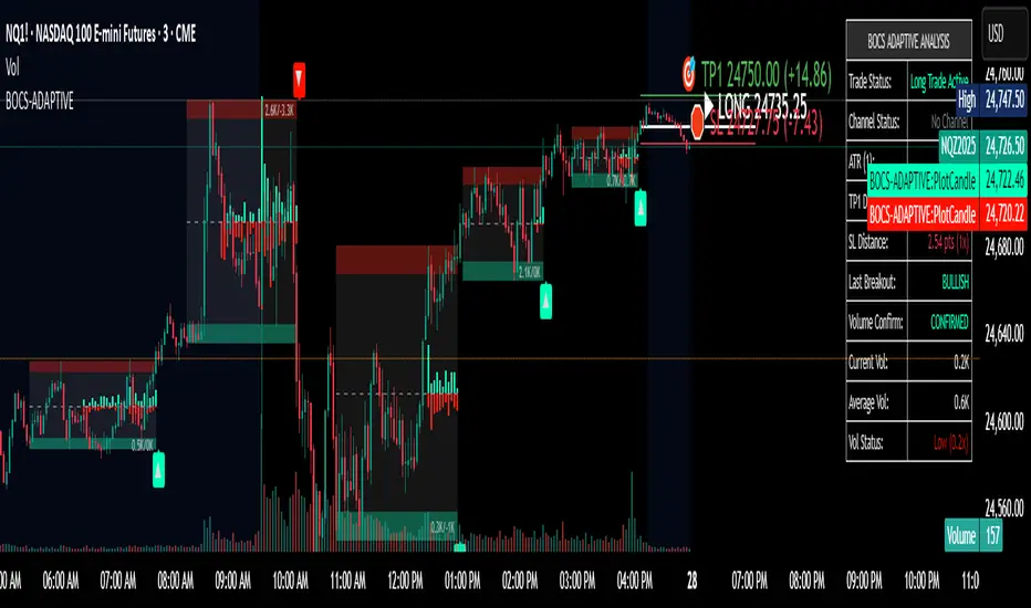
Portfolio Backtester Engine█ OVERVIEW
Portfolio Backtester Engine (PBTE). This tool will allow you to backtest strategies across multiple securities at once. Allowing you to easier understand if your strategy is robust. If you are familiar with the PineCoders backtesting engine , then you will find this indicator pleasant to work with as it is an adaptation based on that work. Much of the functionality has been kept the same, or enhanced, with some minor adjustments I made on the account of creating a more subjectively intuitive tool.
█ HISTORY
The original purpose of the backtesting engine (`BTE`) was to bridge the gap between strategies and studies . Previously, strategies did not contain the ability to send alerts, but were necessary for backtesting. Studies on the other hand were necessary for sending alerts, but could not provide backtesting results . Often, traders would have to manage two separate Pine scripts to take advantage of each feature, this was less than ideal.
The `BTE` published by PineCoders offered a solution to this issue by generating backtesting results under the context of a study(). This allowed traders to backtest their strategy and simultaneously generate alerts for automated trading, thus eliminating the need for a separate strategy() script (though, even converting the engine to a strategy was made simple by the PineCoders!).
Fast forward a couple years and PineScript evolved beyond these issues and alerts were introduced into strategies. The BTE was not quite as necessary anymore, but is still extremely useful as it contains extra features and data not found under the strategy() context. Below is an excerpt of features contained by the BTE:
"""
More than `40` built-in strategies,
Customizable components,
Coupling with your own external indicator,
Simple conversion from Study to Strategy modes,
Post-Exit analysis to search for alternate trade outcomes,
Use of the Data Window to show detailed bar by bar trade information and global statistics, including some not provided by TV backtesting,
Plotting of reminders and generation of alerts on in-trade events.
"""
Before I go any further, I want to be clear that the BTE is STILL a good tool and it is STILL very useful. The Portfolio Backtesting Engine I am introducing is only a tangental advancement and not to be confused as a replacement, this tool would not have been possible without the `BTE`.
█ THE PROBLEM
Most strategies built in Pine are limited by one thing. Data. Backtesting should be a rigorous process and researchers should examine the performance of their strategy across all market regimes; that includes, bullish and bearish markets, ranging markets, low volatility and high volatility. Depending on your TV subscription The Pine Engine is limited to 5k-20k historical bars available for backtesting, which can often leave the strategy results wanting. As a general rule of thumb, strategies should be tested across a quantity of historical bars which will allow for at least 100 trades. In many cases, the lack of historical bars available for backtesting and frequency of the strategy signals produces less than 100 trades, rendering your strategy results inconclusive.
█ THE SOLUTION
In order to be confident that we have a robust strategy we must test it across all market regimes and we must have over 100 trades. To do this effectively, researchers can use the Portfolio Backtesting Engine (PBTE).
By testing a strategy across a carefully selected portfolio of securities, researchers can now gather 5k-20k historical bars per security! Currently, the PTBE allows up to 5 securities, which amounts to 25k-100k historical bars.
█ HOW TO USE
1 — Add the indicator to your chart.
• Confirm inputs. These will be the most important initial values which you can change later by clicking the gear icon ⚙ and opening up the settings of the indicator.
2 — Select a portfolio.
• You will want to spend some time carefully selecting a portfolio of securities.
• Each security should be uncorrelated.
• The entire portfolio should contain a mix of different market regimes.
You should understand that strategies generally take advantage of one particular type of market regime. (trending, ranging, low/high volatility)
For example, the default RSI strategy is typically advantageous during ranging markets, whereas a typical moving average crossover strategy is advantageous in trending markets.
If you were to use the standard RSI strategy during a trending market, you might be selling when you should be buying.
Similarily, if you use an SMA crossover during a ranging market, you will find that the MA's may produce many false signals.
Even if you build a strategy that is designed to be used only in a trending market, it is still best to select a portfolio of all market regimes
as you will be able to test how your strategy will perform when the market does something unexpected.
3 — Test a built-in strategy or add your own.
• Navigate to gear icon ⚙ (settings) of strategy.
• Choose your options.
• Select a Main Entry Strat and Alternate Entry Strat .
• If you want to add your own strategy, you will need to modify the source code and follow the built-in example.
• You will only need to generate (buy 1 / sell -1/ neutral 0) signals.
• Select a Filter , by default these are all off.
• Select an Entry Stop - This will be your stop loss placed at the trade entry.
• Select Pyamiding - This will allow you to stack positions. By default this is off.
• Select Hard Exits - You can also think of these as Take Profits.
• Let the strategy run and take note of the display tables results.
• Portfolio - Shows each security.
• The strategy runs on each asset in your portfolio.
• The initial capital is equally distributed across each security.
So if you have 5 securities and a starting capital of 100,000$ then each security will run the strategy starting with 20,000$
The total row will aggregate the results on a bar by bar basis showing the total results of your initial capital.
• Net Profit (NP) - Shows profitability.
• Number of Trades (#T) - Shows # of trades taken during backtesting period.
• Typically will want to see this number greater than 100 on the "Total" row.
• Average Trade Length (ATL) - Shows average # of days in a trade.
• Maximum Drawdown (MD ) - Max peak-to-valley equity drawdown during backtesting period.
• This number defines the minimum amount of capital required to trade the system.
• Typically, this shouldn’t be lower than 34% and we will want to allow for at least 50% beyond this number.
• Maximum Loss (ML) - Shows largest loss experienced on a per-trade basis.
• Normally, don’t want to exceed more than 1-2 % of equity.
• Maximum Drawdown Duration (MDD) - The longest duration of a drawdown in equity prior to a new equity peak.
• This number is important to help us psychologically understand how long we can expect to wait for a new peak in account equity.
• Maximum Consecutive Losses (MCL) - The max consecutive losses endured throughout the backtesting period.
• Another important metric for trader psychology, this will help you understand how many losses you should be prepared to handle.
• Profit to Maximum Drawdown (P:MD) - A ratio for the average profit to the maximum drawdown.
• The higher the ratio is, the better. Large profits and small losses contribute to a good PMD.
• This metric allows us to examine the profit with respect to risk.
• Profit Loss Ratio (P:L) - Average profit over the average loss.
• Typically this number should be higher in trend following systems.
• Mean reversion systems show lower values, but compensate with a better win %.
• Percent Winners (% W) - The percentage of winning trades.
• Trend systems will usually have lower win percentages, since statistically the market is only trending roughly 30% of the time.
• Mean reversion systems typically should have a high % W.
• Time Percentage (Time %) - The amount of time that the system has an open position.
• The more time you are in the market, the more you are exposed to market risk, not to mention you could be using that money for something else right?
• Return on Investment (ROI) - Your Net Profit over your initial investment, represented as a percentage.
• You want this number to be positive and high.
• Open Profit (OP) - If the strategy has any open positions, the floating value will be represented here.
• Trading Days (TD) - An important metric showing how many days the strategy was active.
• This is good to know and will be valuable in understanding how long you will need to run this strategy in order to achieve results.
█ FEATURES
These are additional features that extend the original `BTE` features.
- Portfolio backtesting.
- Color coded performance results.
- Circuit Breakers that will stop trading.
- Position reversals on exit. (Simulating the function of always in the market. Similar to strategy.entry functionality)
- Whipsaw Filter
- Moving Average Filter
- Minimum Change Filter
- % Gain Equity Exit
- Popular strategies, (MACD, MA cross, supertrend)
Below are features that were excluded from the original `BTE`
- 2 stage in-trade stops with kick-in rules (This was a subjective decision to remove. I found it to be complex and thwarted my use of the `BTE` for some time.)
- Simple conversion from Study to Strategy modes. (Not possible with multiple securities)
- Coupling with your own external indicator (Not really practical to use with multiple securities, but could be used if signals were generated based on some indicator which was not based on the current chart)
- Use of the Data Window to show detailed bar by bar trade information and global statistics.
- Post Exit Analysis.
- Plotting of reminders and generation of alerts on in-trade events.
- Alerts (These may be added in the future by request when I find the time.)
█ THANKS
The whole PineCoders team for all their shared knowledge and original publication of the BTE and Richard Weismann for his ideas on building robust strategies.
═════════════════════════════════════════════════════════════════════════

Kelly Position Size CalculatorThis position sizing calculator implements the Kelly Criterion, developed by John L. Kelly Jr. at Bell Laboratories in 1956, to determine mathematically optimal position sizes for maximizing long-term wealth growth. Unlike arbitrary position sizing methods, this tool provides a scientifically solution based on your strategy's actual performance statistics and incorporates modern refinements from over six decades of academic research.
The Kelly Criterion addresses a fundamental question in capital allocation: "What fraction of capital should be allocated to each opportunity to maximize growth while avoiding ruin?" This question has profound implications for financial markets, where traders and investors constantly face decisions about optimal capital allocation (Van Tharp, 2007).
Theoretical Foundation
The Kelly Criterion for binary outcomes is expressed as f* = (bp - q) / b, where f* represents the optimal fraction of capital to allocate, b denotes the risk-reward ratio, p indicates the probability of success, and q represents the probability of loss (Kelly, 1956). This formula maximizes the expected logarithm of wealth, ensuring maximum long-term growth rate while avoiding the risk of ruin.
The mathematical elegance of Kelly's approach lies in its derivation from information theory. Kelly's original work was motivated by Claude Shannon's information theory (Shannon, 1948), recognizing that maximizing the logarithm of wealth is equivalent to maximizing the rate of information transmission. This connection between information theory and wealth accumulation provides a deep theoretical foundation for optimal position sizing.
The logarithmic utility function underlying the Kelly Criterion naturally embodies several desirable properties for capital management. It exhibits decreasing marginal utility, penalizes large losses more severely than it rewards equivalent gains, and focuses on geometric rather than arithmetic mean returns, which is appropriate for compounding scenarios (Thorp, 2006).
Scientific Implementation
This calculator extends beyond basic Kelly implementation by incorporating state of the art refinements from academic research:
Parameter Uncertainty Adjustment: Following Michaud (1989), the implementation applies Bayesian shrinkage to account for parameter estimation error inherent in small sample sizes. The adjustment formula f_adjusted = f_kelly × confidence_factor + f_conservative × (1 - confidence_factor) addresses the overconfidence bias documented by Baker and McHale (2012), where the confidence factor increases with sample size and the conservative estimate equals 0.25 (quarter Kelly).
Sample Size Confidence: The reliability of Kelly calculations depends critically on sample size. Research by Browne and Whitt (1996) provides theoretical guidance on minimum sample requirements, suggesting that at least 30 independent observations are necessary for meaningful parameter estimates, with 100 or more trades providing reliable estimates for most trading strategies.
Universal Asset Compatibility: The calculator employs intelligent asset detection using TradingView's built-in symbol information, automatically adapting calculations for different asset classes without manual configuration.
ASSET SPECIFIC IMPLEMENTATION
Equity Markets: For stocks and ETFs, position sizing follows the calculation Shares = floor(Kelly Fraction × Account Size / Share Price). This straightforward approach reflects whole share constraints while accommodating fractional share trading capabilities.
Foreign Exchange Markets: Forex markets require lot-based calculations following Lot Size = Kelly Fraction × Account Size / (100,000 × Base Currency Value). The calculator automatically handles major currency pairs with appropriate pip value calculations, following industry standards described by Archer (2010).
Futures Markets: Futures position sizing accounts for leverage and margin requirements through Contracts = floor(Kelly Fraction × Account Size / Margin Requirement). The calculator estimates margin requirements as a percentage of contract notional value, with specific adjustments for micro-futures contracts that have smaller sizes and reduced margin requirements (Kaufman, 2013).
Index and Commodity Markets: These markets combine characteristics of both equity and futures markets. The calculator automatically detects whether instruments are cash-settled or futures-based, applying appropriate sizing methodologies with correct point value calculations.
Risk Management Integration
The calculator integrates sophisticated risk assessment through two primary modes:
Stop Loss Integration: When fixed stop-loss levels are defined, risk calculation follows Risk per Trade = Position Size × Stop Loss Distance. This ensures that the Kelly fraction accounts for actual risk exposure rather than theoretical maximum loss, with stop-loss distance measured in appropriate units for each asset class.
Strategy Drawdown Assessment: For discretionary exit strategies, risk estimation uses maximum historical drawdown through Risk per Trade = Position Value × (Maximum Drawdown / 100). This approach assumes that individual trade losses will not exceed the strategy's historical maximum drawdown, providing a reasonable estimate for strategies with well-defined risk characteristics.
Fractional Kelly Approaches
Pure Kelly sizing can produce substantial volatility, leading many practitioners to adopt fractional Kelly approaches. MacLean, Sanegre, Zhao, and Ziemba (2004) analyze the trade-offs between growth rate and volatility, demonstrating that half-Kelly typically reduces volatility by approximately 75% while sacrificing only 25% of the growth rate.
The calculator provides three primary Kelly modes to accommodate different risk preferences and experience levels. Full Kelly maximizes growth rate while accepting higher volatility, making it suitable for experienced practitioners with strong risk tolerance and robust capital bases. Half Kelly offers a balanced approach popular among professional traders, providing optimal risk-return balance by reducing volatility significantly while maintaining substantial growth potential. Quarter Kelly implements a conservative approach with low volatility, recommended for risk-averse traders or those new to Kelly methodology who prefer gradual introduction to optimal position sizing principles.
Empirical Validation and Performance
Extensive academic research supports the theoretical advantages of Kelly sizing. Hakansson and Ziemba (1995) provide a comprehensive review of Kelly applications in finance, documenting superior long-term performance across various market conditions and asset classes. Estrada (2008) analyzes Kelly performance in international equity markets, finding that Kelly-based strategies consistently outperform fixed position sizing approaches over extended periods across 19 developed markets over a 30-year period.
Several prominent investment firms have successfully implemented Kelly-based position sizing. Pabrai (2007) documents the application of Kelly principles at Berkshire Hathaway, noting Warren Buffett's concentrated portfolio approach aligns closely with Kelly optimal sizing for high-conviction investments. Quantitative hedge funds, including Renaissance Technologies and AQR, have incorporated Kelly-based risk management into their systematic trading strategies.
Practical Implementation Guidelines
Successful Kelly implementation requires systematic application with attention to several critical factors:
Parameter Estimation: Accurate parameter estimation represents the greatest challenge in practical Kelly implementation. Brown (1976) notes that small errors in probability estimates can lead to significant deviations from optimal performance. The calculator addresses this through Bayesian adjustments and confidence measures.
Sample Size Requirements: Users should begin with conservative fractional Kelly approaches until achieving sufficient historical data. Strategies with fewer than 30 trades may produce unreliable Kelly estimates, regardless of adjustments. Full confidence typically requires 100 or more independent trade observations.
Market Regime Considerations: Parameters that accurately describe historical performance may not reflect future market conditions. Ziemba (2003) recommends regular parameter updates and conservative adjustments when market conditions change significantly.
Professional Features and Customization
The calculator provides comprehensive customization options for professional applications:
Multiple Color Schemes: Eight professional color themes (Gold, EdgeTools, Behavioral, Quant, Ocean, Fire, Matrix, Arctic) with dark and light theme compatibility ensure optimal visibility across different trading environments.
Flexible Display Options: Adjustable table size and position accommodate various chart layouts and user preferences, while maintaining analytical depth and clarity.
Comprehensive Results: The results table presents essential information including asset specifications, strategy statistics, Kelly calculations, sample confidence measures, position values, risk assessments, and final position sizes in appropriate units for each asset class.
Limitations and Considerations
Like any analytical tool, the Kelly Criterion has important limitations that users must understand:
Stationarity Assumption: The Kelly Criterion assumes that historical strategy statistics represent future performance characteristics. Non-stationary market conditions may invalidate this assumption, as noted by Lo and MacKinlay (1999).
Independence Requirement: Each trade should be independent to avoid correlation effects. Many trading strategies exhibit serial correlation in returns, which can affect optimal position sizing and may require adjustments for portfolio applications.
Parameter Sensitivity: Kelly calculations are sensitive to parameter accuracy. Regular calibration and conservative approaches are essential when parameter uncertainty is high.
Transaction Costs: The implementation incorporates user-defined transaction costs but assumes these remain constant across different position sizes and market conditions, following Ziemba (2003).
Advanced Applications and Extensions
Multi-Asset Portfolio Considerations: While this calculator optimizes individual position sizes, portfolio-level applications require additional considerations for correlation effects and aggregate risk management. Simplified portfolio approaches include treating positions independently with correlation adjustments.
Behavioral Factors: Behavioral finance research reveals systematic biases that can interfere with Kelly implementation. Kahneman and Tversky (1979) document loss aversion, overconfidence, and other cognitive biases that lead traders to deviate from optimal strategies. Successful implementation requires disciplined adherence to calculated recommendations.
Time-Varying Parameters: Advanced implementations may incorporate time-varying parameter models that adjust Kelly recommendations based on changing market conditions, though these require sophisticated econometric techniques and substantial computational resources.
Comprehensive Usage Instructions and Practical Examples
Implementation begins with loading the calculator on your desired trading instrument's chart. The system automatically detects asset type across stocks, forex, futures, and cryptocurrency markets while extracting current price information. Navigation to the indicator settings allows input of your specific strategy parameters.
Strategy statistics configuration requires careful attention to several key metrics. The win rate should be calculated from your backtest results using the formula of winning trades divided by total trades multiplied by 100. Average win represents the sum of all profitable trades divided by the number of winning trades, while average loss calculates the sum of all losing trades divided by the number of losing trades, entered as a positive number. The total historical trades parameter requires the complete number of trades in your backtest, with a minimum of 30 trades recommended for basic functionality and 100 or more trades optimal for statistical reliability. Account size should reflect your available trading capital, specifically the risk capital allocated for trading rather than total net worth.
Risk management configuration adapts to your specific trading approach. The stop loss setting should be enabled if you employ fixed stop-loss exits, with the stop loss distance specified in appropriate units depending on the asset class. For stocks, this distance is measured in dollars, for forex in pips, and for futures in ticks. When stop losses are not used, the maximum strategy drawdown percentage from your backtest provides the risk assessment baseline. Kelly mode selection offers three primary approaches: Full Kelly for aggressive growth with higher volatility suitable for experienced practitioners, Half Kelly for balanced risk-return optimization popular among professional traders, and Quarter Kelly for conservative approaches with reduced volatility.
Display customization ensures optimal integration with your trading environment. Eight professional color themes provide optimization for different chart backgrounds and personal preferences. Table position selection allows optimal placement within your chart layout, while table size adjustment ensures readability across different screen resolutions and viewing preferences.
Detailed Practical Examples
Example 1: SPY Swing Trading Strategy
Consider a professionally developed swing trading strategy for SPY (S&P 500 ETF) with backtesting results spanning 166 total trades. The strategy achieved 110 winning trades, representing a 66.3% win rate, with an average winning trade of $2,200 and average losing trade of $862. The maximum drawdown reached 31.4% during the testing period, and the available trading capital amounts to $25,000. This strategy employs discretionary exits without fixed stop losses.
Implementation requires loading the calculator on the SPY daily chart and configuring the parameters accordingly. The win rate input receives 66.3, while average win and loss inputs receive 2200 and 862 respectively. Total historical trades input requires 166, with account size set to 25000. The stop loss function remains disabled due to the discretionary exit approach, with maximum strategy drawdown set to 31.4%. Half Kelly mode provides the optimal balance between growth and risk management for this application.
The calculator generates several key outputs for this scenario. The risk-reward ratio calculates automatically to 2.55, while the Kelly fraction reaches approximately 53% before scientific adjustments. Sample confidence achieves 100% given the 166 trades providing high statistical confidence. The recommended position settles at approximately 27% after Half Kelly and Bayesian adjustment factors. Position value reaches approximately $6,750, translating to 16 shares at a $420 SPY price. Risk per trade amounts to approximately $2,110, representing 31.4% of position value, with expected value per trade reaching approximately $1,466. This recommendation represents the mathematically optimal balance between growth potential and risk management for this specific strategy profile.
Example 2: EURUSD Day Trading with Stop Losses
A high-frequency EURUSD day trading strategy demonstrates different parameter requirements compared to swing trading approaches. This strategy encompasses 89 total trades with a 58% win rate, generating an average winning trade of $180 and average losing trade of $95. The maximum drawdown reached 12% during testing, with available capital of $10,000. The strategy employs fixed stop losses at 25 pips and take profit targets at 45 pips, providing clear risk-reward parameters.
Implementation begins with loading the calculator on the EURUSD 1-hour chart for appropriate timeframe alignment. Parameter configuration includes win rate at 58, average win at 180, and average loss at 95. Total historical trades input receives 89, with account size set to 10000. The stop loss function is enabled with distance set to 25 pips, reflecting the fixed exit strategy. Quarter Kelly mode provides conservative positioning due to the smaller sample size compared to the previous example.
Results demonstrate the impact of smaller sample sizes on Kelly calculations. The risk-reward ratio calculates to 1.89, while the Kelly fraction reaches approximately 32% before adjustments. Sample confidence achieves 89%, providing moderate statistical confidence given the 89 trades. The recommended position settles at approximately 7% after Quarter Kelly application and Bayesian shrinkage adjustment for the smaller sample. Position value amounts to approximately $700, translating to 0.07 standard lots. Risk per trade reaches approximately $175, calculated as 25 pips multiplied by lot size and pip value, with expected value per trade at approximately $49. This conservative position sizing reflects the smaller sample size, with position sizes expected to increase as trade count surpasses 100 and statistical confidence improves.
Example 3: ES1! Futures Systematic Strategy
Systematic futures trading presents unique considerations for Kelly criterion application, as demonstrated by an E-mini S&P 500 futures strategy encompassing 234 total trades. This systematic approach achieved a 45% win rate with an average winning trade of $1,850 and average losing trade of $720. The maximum drawdown reached 18% during the testing period, with available capital of $50,000. The strategy employs 15-tick stop losses with contract specifications of $50 per tick, providing precise risk control mechanisms.
Implementation involves loading the calculator on the ES1! 15-minute chart to align with the systematic trading timeframe. Parameter configuration includes win rate at 45, average win at 1850, and average loss at 720. Total historical trades receives 234, providing robust statistical foundation, with account size set to 50000. The stop loss function is enabled with distance set to 15 ticks, reflecting the systematic exit methodology. Half Kelly mode balances growth potential with appropriate risk management for futures trading.
Results illustrate how favorable risk-reward ratios can support meaningful position sizing despite lower win rates. The risk-reward ratio calculates to 2.57, while the Kelly fraction reaches approximately 16%, lower than previous examples due to the sub-50% win rate. Sample confidence achieves 100% given the 234 trades providing high statistical confidence. The recommended position settles at approximately 8% after Half Kelly adjustment. Estimated margin per contract amounts to approximately $2,500, resulting in a single contract allocation. Position value reaches approximately $2,500, with risk per trade at $750, calculated as 15 ticks multiplied by $50 per tick. Expected value per trade amounts to approximately $508. Despite the lower win rate, the favorable risk-reward ratio supports meaningful position sizing, with single contract allocation reflecting appropriate leverage management for futures trading.
Example 4: MES1! Micro-Futures for Smaller Accounts
Micro-futures contracts provide enhanced accessibility for smaller trading accounts while maintaining identical strategy characteristics. Using the same systematic strategy statistics from the previous example but with available capital of $15,000 and micro-futures specifications of $5 per tick with reduced margin requirements, the implementation demonstrates improved position sizing granularity.
Kelly calculations remain identical to the full-sized contract example, maintaining the same risk-reward dynamics and statistical foundations. However, estimated margin per contract reduces to approximately $250 for micro-contracts, enabling allocation of 4-5 micro-contracts. Position value reaches approximately $1,200, while risk per trade calculates to $75, derived from 15 ticks multiplied by $5 per tick. This granularity advantage provides better position size precision for smaller accounts, enabling more accurate Kelly implementation without requiring large capital commitments.
Example 5: Bitcoin Swing Trading
Cryptocurrency markets present unique challenges requiring modified Kelly application approaches. A Bitcoin swing trading strategy on BTCUSD encompasses 67 total trades with a 71% win rate, generating average winning trades of $3,200 and average losing trades of $1,400. Maximum drawdown reached 28% during testing, with available capital of $30,000. The strategy employs technical analysis for exits without fixed stop losses, relying on price action and momentum indicators.
Implementation requires conservative approaches due to cryptocurrency volatility characteristics. Quarter Kelly mode is recommended despite the high win rate to account for crypto market unpredictability. Expected position sizing remains reduced due to the limited sample size of 67 trades, requiring additional caution until statistical confidence improves. Regular parameter updates are strongly recommended due to cryptocurrency market evolution and changing volatility patterns that can significantly impact strategy performance characteristics.
Advanced Usage Scenarios
Portfolio position sizing requires sophisticated consideration when running multiple strategies simultaneously. Each strategy should have its Kelly fraction calculated independently to maintain mathematical integrity. However, correlation adjustments become necessary when strategies exhibit related performance patterns. Moderately correlated strategies should receive individual position size reductions of 10-20% to account for overlapping risk exposure. Aggregate portfolio risk monitoring ensures total exposure remains within acceptable limits across all active strategies. Professional practitioners often consider using lower fractional Kelly approaches, such as Quarter Kelly, when running multiple strategies simultaneously to provide additional safety margins.
Parameter sensitivity analysis forms a critical component of professional Kelly implementation. Regular validation procedures should include monthly parameter updates using rolling 100-trade windows to capture evolving market conditions while maintaining statistical relevance. Sensitivity testing involves varying win rates by ±5% and average win/loss ratios by ±10% to assess recommendation stability under different parameter assumptions. Out-of-sample validation reserves 20% of historical data for parameter verification, ensuring that optimization doesn't create curve-fitted results. Regime change detection monitors actual performance against expected metrics, triggering parameter reassessment when significant deviations occur.
Risk management integration requires professional overlay considerations beyond pure Kelly calculations. Daily loss limits should cease trading when daily losses exceed twice the calculated risk per trade, preventing emotional decision-making during adverse periods. Maximum position limits should never exceed 25% of account value in any single position regardless of Kelly recommendations, maintaining diversification principles. Correlation monitoring reduces position sizes when holding multiple correlated positions that move together during market stress. Volatility adjustments consider reducing position sizes during periods of elevated VIX above 25 for equity strategies, adapting to changing market conditions.
Troubleshooting and Optimization
Professional implementation often encounters specific challenges requiring systematic troubleshooting approaches. Zero position size displays typically result from insufficient capital for minimum position sizes, negative expected values, or extremely conservative Kelly calculations. Solutions include increasing account size, verifying strategy statistics for accuracy, considering Quarter Kelly mode for conservative approaches, or reassessing overall strategy viability when fundamental issues exist.
Extremely high Kelly fractions exceeding 50% usually indicate underlying problems with parameter estimation. Common causes include unrealistic win rates, inflated risk-reward ratios, or curve-fitted backtest results that don't reflect genuine trading conditions. Solutions require verifying backtest methodology, including all transaction costs in calculations, testing strategies on out-of-sample data, and using conservative fractional Kelly approaches until parameter reliability improves.
Low sample confidence below 50% reflects insufficient historical trades for reliable parameter estimation. This situation demands gathering additional trading data, using Quarter Kelly approaches until reaching 100 or more trades, applying extra conservatism in position sizing, and considering paper trading to build statistical foundations without capital risk.
Inconsistent results across similar strategies often stem from parameter estimation differences, market regime changes, or strategy degradation over time. Professional solutions include standardizing backtest methodology across all strategies, updating parameters regularly to reflect current conditions, and monitoring live performance against expectations to identify deteriorating strategies.
Position sizes that appear inappropriately large or small require careful validation against traditional risk management principles. Professional standards recommend never risking more than 2-3% per trade regardless of Kelly calculations. Calibration should begin with Quarter Kelly approaches, gradually increasing as comfort and confidence develop. Most institutional traders utilize 25-50% of full Kelly recommendations to balance growth with prudent risk management.
Market condition adjustments require dynamic approaches to Kelly implementation. Trending markets may support full Kelly recommendations when directional momentum provides favorable conditions. Ranging or volatile markets typically warrant reducing to Half or Quarter Kelly to account for increased uncertainty. High correlation periods demand reducing individual position sizes when multiple positions move together, concentrating risk exposure. News and event periods often justify temporary position size reductions during high-impact releases that can create unpredictable market movements.
Performance monitoring requires systematic protocols to ensure Kelly implementation remains effective over time. Weekly reviews should compare actual versus expected win rates and average win/loss ratios to identify parameter drift or strategy degradation. Position size efficiency and execution quality monitoring ensures that calculated recommendations translate effectively into actual trading results. Tracking correlation between calculated and realized risk helps identify discrepancies between theoretical and practical risk exposure.
Monthly calibration provides more comprehensive parameter assessment using the most recent 100 trades to maintain statistical relevance while capturing current market conditions. Kelly mode appropriateness requires reassessment based on recent market volatility and performance characteristics, potentially shifting between Full, Half, and Quarter Kelly approaches as conditions change. Transaction cost evaluation ensures that commission structures, spreads, and slippage estimates remain accurate and current.
Quarterly strategic reviews encompass comprehensive strategy performance analysis comparing long-term results against expectations and identifying trends in effectiveness. Market regime assessment evaluates parameter stability across different market conditions, determining whether strategy characteristics remain consistent or require fundamental adjustments. Strategic modifications to position sizing methodology may become necessary as markets evolve or trading approaches mature, ensuring that Kelly implementation continues supporting optimal capital allocation objectives.
Professional Applications
This calculator serves diverse professional applications across the financial industry. Quantitative hedge funds utilize the implementation for systematic position sizing within algorithmic trading frameworks, where mathematical precision and consistent application prove essential for institutional capital management. Professional discretionary traders benefit from optimized position management that removes emotional bias while maintaining flexibility for market-specific adjustments. Portfolio managers employ the calculator for developing risk-adjusted allocation strategies that enhance returns while maintaining prudent risk controls across diverse asset classes and investment strategies.
Individual traders seeking mathematical optimization of capital allocation find the calculator provides institutional-grade methodology previously available only to professional money managers. The Kelly Criterion establishes theoretical foundation for optimal capital allocation across both single strategies and multiple trading systems, offering significant advantages over arbitrary position sizing methods that rely on intuition or fixed percentage approaches. Professional implementation ensures consistent application of mathematically sound principles while adapting to changing market conditions and strategy performance characteristics.
Conclusion
The Kelly Criterion represents one of the few mathematically optimal solutions to fundamental investment problems. When properly understood and carefully implemented, it provides significant competitive advantage in financial markets. This calculator implements modern refinements to Kelly's original formula while maintaining accessibility for practical trading applications.
Success with Kelly requires ongoing learning, systematic application, and continuous refinement based on market feedback and evolving research. Users who master Kelly principles and implement them systematically can expect superior risk-adjusted returns and more consistent capital growth over extended periods.
The extensive academic literature provides rich resources for deeper study, while practical experience builds the intuition necessary for effective implementation. Regular parameter updates, conservative approaches with limited data, and disciplined adherence to calculated recommendations are essential for optimal results.
References
Archer, M. D. (2010). Getting Started in Currency Trading: Winning in Today's Forex Market (3rd ed.). John Wiley & Sons.
Baker, R. D., & McHale, I. G. (2012). An empirical Bayes approach to optimising betting strategies. Journal of the Royal Statistical Society: Series D (The Statistician), 61(1), 75-92.
Breiman, L. (1961). Optimal gambling systems for favorable games. In J. Neyman (Ed.), Proceedings of the Fourth Berkeley Symposium on Mathematical Statistics and Probability (pp. 65-78). University of California Press.
Brown, D. B. (1976). Optimal portfolio growth: Logarithmic utility and the Kelly criterion. In W. T. Ziemba & R. G. Vickson (Eds.), Stochastic Optimization Models in Finance (pp. 1-23). Academic Press.
Browne, S., & Whitt, W. (1996). Portfolio choice and the Bayesian Kelly criterion. Advances in Applied Probability, 28(4), 1145-1176.
Estrada, J. (2008). Geometric mean maximization: An overlooked portfolio approach? The Journal of Investing, 17(4), 134-147.
Hakansson, N. H., & Ziemba, W. T. (1995). Capital growth theory. In R. A. Jarrow, V. Maksimovic, & W. T. Ziemba (Eds.), Handbooks in Operations Research and Management Science (Vol. 9, pp. 65-86). Elsevier.
Kahneman, D., & Tversky, A. (1979). Prospect theory: An analysis of decision under risk. Econometrica, 47(2), 263-291.
Kaufman, P. J. (2013). Trading Systems and Methods (5th ed.). John Wiley & Sons.
Kelly Jr, J. L. (1956). A new interpretation of information rate. Bell System Technical Journal, 35(4), 917-926.
Lo, A. W., & MacKinlay, A. C. (1999). A Non-Random Walk Down Wall Street. Princeton University Press.
MacLean, L. C., Sanegre, E. O., Zhao, Y., & Ziemba, W. T. (2004). Capital growth with security. Journal of Economic Dynamics and Control, 28(4), 937-954.
MacLean, L. C., Thorp, E. O., & Ziemba, W. T. (2011). The Kelly Capital Growth Investment Criterion: Theory and Practice. World Scientific.
Michaud, R. O. (1989). The Markowitz optimization enigma: Is 'optimized' optimal? Financial Analysts Journal, 45(1), 31-42.
Pabrai, M. (2007). The Dhandho Investor: The Low-Risk Value Method to High Returns. John Wiley & Sons.
Shannon, C. E. (1948). A mathematical theory of communication. Bell System Technical Journal, 27(3), 379-423.
Tharp, V. K. (2007). Trade Your Way to Financial Freedom (2nd ed.). McGraw-Hill.
Thorp, E. O. (2006). The Kelly criterion in blackjack sports betting, and the stock market. In L. C. MacLean, E. O. Thorp, & W. T. Ziemba (Eds.), The Kelly Capital Growth Investment Criterion: Theory and Practice (pp. 789-832). World Scientific.
Van Tharp, K. (2007). Trade Your Way to Financial Freedom (2nd ed.). McGraw-Hill Education.
Vince, R. (1992). The Mathematics of Money Management: Risk Analysis Techniques for Traders. John Wiley & Sons.
Vince, R., & Zhu, H. (2015). Optimal betting under parameter uncertainty. Journal of Statistical Planning and Inference, 161, 19-31.
Ziemba, W. T. (2003). The Stochastic Programming Approach to Asset, Liability, and Wealth Management. The Research Foundation of AIMR.
Further Reading
For comprehensive understanding of Kelly Criterion applications and advanced implementations:
MacLean, L. C., Thorp, E. O., & Ziemba, W. T. (2011). The Kelly Capital Growth Investment Criterion: Theory and Practice. World Scientific.
Vince, R. (1992). The Mathematics of Money Management: Risk Analysis Techniques for Traders. John Wiley & Sons.
Thorp, E. O. (2017). A Man for All Markets: From Las Vegas to Wall Street. Random House.
Cover, T. M., & Thomas, J. A. (2006). Elements of Information Theory (2nd ed.). John Wiley & Sons.
Ziemba, W. T., & Vickson, R. G. (Eds.). (2006). Stochastic Optimization Models in Finance. World Scientific.

Superior-Range Bound Renko - Alerts - 11-29-25 - Signal LynxSuperior-Range Bound Renko – Alerts Edition with Advanced Risk Management Template
Signal Lynx | Free Scripts supporting Automation for the Night-Shift Nation 🌙
1. Overview
This is the Alerts & Indicator Edition of Superior-Range Bound Renko (RBR).
The Strategy version is built for backtesting inside TradingView.
This Alerts version is built for automation: it emits clean, discrete alert events that you can route into webhooks, bots, or relay engines (including your own Signal Lynx-style infrastructure).
Under the hood, this script contains the same core engine as the strategy:
Adaptive Range Bounding based on volatility
Renko Brick Emulation on standard candles
A stack of Laguerre Filters for impulse detection
K-Means-style Adaptive SuperTrend for trend confirmation
The full Signal Lynx Risk Management Engine (state machine, layered exits, AATS, RSIS, etc.)
The difference is in what we output:
Instead of placing historical trades, this version:
Plots the entry and RM signals in a separate pane (overlay = false)
Exposes alertconditions for:
Long Entry
Short Entry
Close Long
Close Short
TP1, TP2, TP3 hits (Staged Take Profit)
This makes it ideal as the signal source for automated execution via TradingView Alerts + Webhooks.
2. Quick Action Guide (TL;DR)
Best Timeframe:
4H and above. This is a swing-trading / position-trading style engine, not a micro-scalper.
Best Assets:
Volatile but structured markets, e.g.:
BTC, ETH, XAUUSD (Gold), GBPJPY, and similar high-volatility majors or indices.
Script Type:
indicator() – Alerts & Visualization Only
No built-in order placement
All “orders” are emitted as alerts for your external bot or manual handling
Strategy Type:
Volatility-Adaptive Trend Following + Impulse Detection
using Renko-like structure and multi-layer Laguerre filters.
Repainting:
Designed to be non-repainting on closed candles.
The underlying Risk Management engine is built around previous-bar data (close , high , low ) for execution-critical logic.
Intrabar values can move while the bar is forming (normal for any advanced signal), but once a bar closes, the alert logic is stable.
Recommended Alert Settings:
Condition: one of the built-in signals (see section 3.B)
Options: “Once Per Bar Close” is strongly recommended for automation
Message: JSON, CSV, or simple tokens – whatever your webhook / relay expects
3. Detailed Report: How the Alerts Edition Works
A. Relationship to the Strategy Version
The Alerts Edition shares the same internal logic as the strategy version:
Same Adaptive Lookback and volatility normalization
Same Range and Close Range construction
Same Renko Brick Emulator and directional memory (renkoDir)
Same Fib structures, Laguerre stack, K-Means SuperTrend, and Baseline signals (B1, B2)
Same Risk Management Engine and layered exits
In the strategy script, these signals are wired into strategy.entry, strategy.exit, and strategy.close.
In the alerts script:
We still compute the final entry/exit signals (Fin, CloseEmAll, TakeProfit1Plot, etc.)
Instead of placing trades, we:
Plot them for visual inspection
Expose them via alertcondition(...) so that TradingView can fire alerts.
This ensures that:
If you use the same settings on the same symbol/timeframe, the Alerts Edition and Strategy Edition agree on where entries and exits occur.
(Subject only to normal intrabar vs. bar-close differences.)
B. Signals & Alert Conditions
The alerts script focuses on discrete, automation-friendly events.
Internally, the main signals are:
Fin – Final entry decision from the RM engine
CloseEmAll – RM-driven “hard close” signal (for full-position exits)
TakeProfit1Plot / 2Plot / 3Plot – One-time event markers when each TP stage is hit
On the chart (in the separate indicator pane), you get:
plot(Fin) – where:
+2 = Long Entry event
-2 = Short Entry event
plot(CloseEmAll) – where:
+1 = “Close Long” event
-1 = “Close Short” event
plot(TP1/TP2/TP3) (if Staged TP is enabled) – integer tags for TP hits:
+1 / +2 / +3 = TP1 / TP2 / TP3 for Longs
-1 / -2 / -3 = TP1 / TP2 / TP3 for Shorts
The corresponding alertconditions are:
Long Entry
alertcondition(Fin == 2, title="Long Entry", message="Long Entry Triggered")
Fire this to open/scale a long position in your bot.
Short Entry
alertcondition(Fin == -2, title="Short Entry", message="Short Entry Triggered")
Fire this to open/scale a short position.
Close Long
alertcondition(CloseEmAll == 1, title="Close Long", message="Close Long Triggered")
Fire this to fully exit a long position.
Close Short
alertcondition(CloseEmAll == -1, title="Close Short", message="Close Short Triggered")
Fire this to fully exit a short position.
TP 1 Hit
alertcondition(TakeProfit1Plot != 0, title="TP 1 Hit", message="TP 1 Level Reached")
First staged take profit hit (either long or short). Your bot can interpret the direction based on position state or message tags.
TP 2 Hit
alertcondition(TakeProfit2Plot != 0, title="TP 2 Hit", message="TP 2 Level Reached")
TP 3 Hit
alertcondition(TakeProfit3Plot != 0, title="TP 3 Hit", message="TP 3 Level Reached")
Together, these give you a complete trade lifecycle:
Open Long / Short
Optionally scale out via TP1/TP2/TP3
Close remaining via Close Long / Close Short
All while the Risk Management Engine enforces the same logic as the strategy version.
C. Using This Script for Automation
This Alerts Edition is designed for:
Webhook-based bots
Execution relays (e.g., your own Lynx-Relay-style engine)
Dedicated external trade managers
Typical setup flow:
Add the script to your chart
Same symbol, timeframe, and settings you use in the Strategy Edition backtests.
Configure Inputs:
Longs / Shorts enabled
Risk Management toggles (SL, TS, Staged TP, AATS, RSIS)
Weekend filter (if you do not want weekend trades)
RBR-specific knobs (Adaptive Lookback, Brick type, ATR vs Standard Brick, etc.)
Create Alerts for Each Event Type You Need:
Long Entry
Short Entry
Close Long
Close Short
TP1 / TP2 / TP3 (optional, if your bot handles partial closes)
For each:
Condition: the corresponding alertcondition
Option: “Once Per Bar Close” is strongly recommended
Message:
You can use structured JSON or a simple token set like:
{"side":"long","event":"entry","symbol":"{{ticker}}","time":"{{timenow}}"}
or a simpler text for manual trading like:
LONG ENTRY | {{ticker}} | {{interval}}
Wire Up Your Bot / Relay:
Point TradingView’s webhook URL to your execution engine
Parse the messages and map them into:
Exchange
Symbol
Side (long/short)
Action (open/close/partial)
Size and risk model (this script does not position-size for you; it only signals when, not how much.)
Because the alerts come from a non-repainting, RM-backed engine that you’ve already validated via the Strategy Edition, you get a much cleaner automation pipeline.
D. Repainting Protection (Alerts Edition)
The same protections as the Strategy Edition apply here:
Execution-critical logic (trailing stop, TP triggers, SL, RM state changes) uses previous bar OHLC:
open , high , low , close
No security() with lookahead or future-bar dependencies.
This means:
Alerts are designed to fire on states that would have been visible at bar close, not on hypothetical “future history.”
Important practical note:
Intrabar: While a bar is forming, internal conditions can oscillate.
Bar Close: With “Once Per Bar Close” alerts, the fired signal corresponds to the final state of the engine for that candle, matching your Strategy Edition expectations.
4. For Developers & Modders
You can treat this Alerts script as an ”RM + Alert Framework” and inject any signal logic you want.
Where to plug in:
Find the section:
// BASELINE & SIGNAL GENERATION
You’ll see how B1 and B2 are built from the RBR stack and then combined:
baseSig = B2
altSig = B1
finalSig = sigSwap ? baseSig : altSig
To use your own logic:
Replace or wrap the code that sets baseSig / altSig with your own conditions:
e.g., RSI, MACD, Heikin Ashi filters, candle patterns, volume filters, etc.
Make sure your final decision is still:
2 → Long / Buy signal
-2 → Short / Sell signal
0 → No trade
finalSig is then passed into the RM engine and eventually becomes Fin, which:
Drives the Long/Short Entry alerts
Interacts with the RM state machine to integrate properly with AATS, SL, TS, TP, etc.
Because this script already exposes alertconditions for key lifecycle events, you don’t need to re-wire alerts each time — just ensure your logic feeds into finalSig correctly.
This lets you use the Signal Lynx Risk Management Engine + Alerts wrapper as a drop-in chassis for your own strategies.
5. About Signal Lynx
Automation for the Night-Shift Nation 🌙
Signal Lynx builds tools and templates that help traders move from:
“I have an indicator” → “I have a structured, automatable strategy with real risk management.”
This Superior-Range Bound Renko – Alerts Edition is the automation-focused companion to the Strategy Edition. It’s designed for:
Traders who backtest with the Strategy version
Then deploy live signals with this Alerts version via webhooks or bots
While relying on the same non-repainting, RM-driven logic
We release this code under the Mozilla Public License 2.0 (MPL-2.0) to support the Pine community with:
Transparent, inspectable logic
A reusable Risk Management template
A reference implementation of advanced adaptive logic + alerts
If you are exploring full-stack automation (TradingView → Webhooks → Exchange / VPS), keep Signal Lynx in your search.
License: Mozilla Public License 2.0 (Open Source).
If you build improvements or helpful variants, please consider sharing them back with the community.

J.P. Morgan Efficiente 5 IndexJ.P. MORGAN EFFICIENTE 5 INDEX REPLICATION
Walk into any retail trading forum and you'll find the same scene playing out thousands of times a day: traders huddled over their screens, drawing trendlines on candlestick charts, hunting for the perfect entry signal, convinced that the next RSI crossover will unlock the path to financial freedom. Meanwhile, in the towers of lower Manhattan and the City of London, portfolio managers are doing something entirely different. They're not drawing lines. They're not hunting patterns. They're building fortresses of diversification, wielding mathematical frameworks that have survived decades of market chaos, and most importantly, they're thinking in portfolios while retail thinks in positions.
This divide is not just philosophical. It's structural, mathematical, and ultimately, profitable. The uncomfortable truth that retail traders must confront is this: while you're obsessing over whether the 50-day moving average will cross the 200-day, institutional investors are solving quadratic optimization problems across thirteen asset classes, rebalancing monthly according to Markowitz's Nobel Prize-winning framework, and targeting precise volatility levels that allow them to sleep at night regardless of what the VIX does tomorrow. The game you're playing and the game they're playing share the same field, but the rules are entirely different.
The question, then, is not whether retail traders can access institutional strategies. The question is whether they're willing to fundamentally change how they think about markets. Are you ready to stop painting lines and start building portfolios?
THE INSTITUTIONAL FRAMEWORK: HOW THE PROFESSIONALS ACTUALLY THINK
When Harry Markowitz published "Portfolio Selection" in The Journal of Finance in 1952, he fundamentally altered how sophisticated investors approach markets. His insight was deceptively simple: returns alone mean nothing. Risk-adjusted returns mean everything. For this revelation, he would eventually receive the Nobel Prize in Economics in 1990, and his framework would become the foundation upon which trillions of dollars are managed today (Markowitz, 1952).
Modern Portfolio Theory, as it came to be known, introduced a revolutionary concept: through diversification across imperfectly correlated assets, an investor could reduce portfolio risk without sacrificing expected returns. This wasn't about finding the single best asset. It was about constructing the optimal combination of assets. The mathematics are elegant in their logic: if two assets don't move in perfect lockstep, combining them creates a portfolio whose volatility is lower than the weighted average of the individual volatilities. This "free lunch" of diversification became the bedrock of institutional investment management (Elton et al., 2014).
But here's where retail traders miss the point entirely: this isn't about having ten different stocks instead of one. It's about systematic, mathematically rigorous allocation across asset classes with fundamentally different risk drivers. When equity markets crash, high-quality government bonds often rally. When inflation surges, commodities may provide protection even as stocks and bonds both suffer. When emerging markets are in vogue, developed markets may lag. The professional investor doesn't predict which scenario will unfold. Instead, they position for all of them simultaneously, with weights determined not by gut feeling but by quantitative optimization.
This is what J.P. Morgan Asset Management embedded into their Efficiente Index series. These are not actively managed funds where a portfolio manager makes discretionary calls. They are rules-based, systematic strategies that execute the Markowitz framework in real-time, rebalancing monthly to maintain optimal risk-adjusted positioning across global equities, fixed income, commodities, and defensive assets (J.P. Morgan Asset Management, 2016).
THE EFFICIENTE 5 STRATEGY: DECONSTRUCTING INSTITUTIONAL METHODOLOGY
The Efficiente 5 Index, specifically, targets a 5% annualized volatility. Let that sink in for a moment. While retail traders routinely accept 20%, 30%, or even 50% annual volatility in pursuit of returns, institutional allocators have determined that 5% volatility provides an optimal balance between growth potential and capital preservation. This isn't timidity. It's mathematics. At higher volatility levels, the compounding drag from large drawdowns becomes mathematically punishing. A 50% loss requires a 100% gain just to break even. The institutional solution: constrain volatility at the portfolio level, allowing the power of compounding to work unimpeded (Damodaran, 2008).
The strategy operates across thirteen exchange-traded funds spanning five distinct asset classes: developed equity markets (SPY, IWM, EFA), fixed income across the risk spectrum (TLT, LQD, HYG), emerging markets (EEM, EMB), alternatives (IYR, GSG, GLD), and defensive positioning (TIP, BIL). These aren't arbitrary choices. Each ETF represents a distinct factor exposure, and together they provide access to the primary drivers of global asset returns (Fama and French, 1993).
The methodology, as detailed in replication research by Jungle Rock (2025), follows a precise monthly cadence. At the end of each month, the strategy recalculates expected returns and volatilities for all thirteen assets using a 126-day rolling window. This six-month lookback balances responsiveness to changing market conditions against the noise of short-term fluctuations. The optimization engine then solves for the portfolio weights that maximize expected return subject to the 5% volatility target, with additional constraints to prevent excessive concentration.
These constraints are critical and reveal institutional wisdom that retail traders typically ignore. No single ETF can exceed 20% of the portfolio, except for TIP and BIL which can reach 50% given their defensive nature. At the asset class level, developed equities are capped at 50%, bonds at 50%, emerging markets at 25%, and alternatives at 25%. These aren't arbitrary limits. They're guardrails preventing the optimization from becoming too aggressive during periods when recent performance might suggest concentrating heavily in a single area that's been hot (Jorion, 1992).
After optimization, there's one final step that appears almost trivial but carries profound implications: weights are rounded to the nearest 5%. In a world of fractional shares and algorithmic execution, why round to 5%? The answer reveals institutional practicality over mathematical purity. A portfolio weight of 13.7% and 15.0% are functionally similar in their risk contribution, but the latter is vastly easier to communicate, to monitor, and to execute at scale. When you're managing billions, parsimony matters.
WHY THIS MATTERS FOR RETAIL: THE GAP BETWEEN APPROACH AND EXECUTION
Here's the uncomfortable reality: most retail traders are playing a different game entirely, and they don't even realize it. When a retail trader says "I'm bullish on tech," they buy QQQ and that's their entire technology exposure. When they say "I need some diversification," they buy ten different stocks, often in correlated sectors. This isn't diversification in the Markowitzian sense. It's concentration with extra steps.
The institutional approach represented by the Efficiente 5 is fundamentally different in several ways. First, it's systematic. Emotions don't drive the allocation. The mathematics do. When equities have rallied hard and now represent 55% of the portfolio despite a 50% cap, the system sells equities and buys bonds or alternatives, regardless of how bullish the headlines feel. This forced contrarianism is what retail traders know they should do but rarely execute (Kahneman and Tversky, 1979).
Second, it's forward-looking in its inputs but backward-looking in its process. The strategy doesn't try to predict the next crisis or the next boom. It simply measures what volatility and returns have been recently, assumes the immediate future resembles the immediate past more than it resembles some forecast, and positions accordingly. This humility regarding prediction is perhaps the most institutional characteristic of all.
Third, and most critically, it treats the portfolio as a single organism. Retail traders typically view their holdings as separate positions, each requiring individual management. The institutional approach recognizes that what matters is not whether Position A made money, but whether the portfolio as a whole achieved its risk-adjusted return target. A position can lose money and still be a valuable contributor if it reduced portfolio volatility or provided diversification during stress periods.
THE MATHEMATICAL FOUNDATION: MEAN-VARIANCE OPTIMIZATION IN PRACTICE
At its core, the Efficiente 5 strategy solves a constrained optimization problem each month. In technical terms, this is a quadratic programming problem: maximize expected portfolio return subject to a volatility constraint and position limits. The objective function is straightforward: maximize the weighted sum of expected returns. The constraint is that the weighted sum of variances and covariances must not exceed the volatility target squared (Markowitz, 1959).
The challenge, and this is crucial for understanding the Pine Script implementation, is that solving this problem properly requires calculating a covariance matrix. This 13x13 matrix captures not just the volatility of each asset but the correlation between every pair of assets. Two assets might each have 15% volatility, but if they're negatively correlated, combining them reduces portfolio risk. If they're positively correlated, it doesn't. The covariance matrix encodes these relationships.
True mean-variance optimization requires matrix algebra and quadratic programming solvers. Pine Script, by design, lacks these capabilities. The language doesn't support matrix operations, and certainly doesn't include a QP solver. This creates a fundamental challenge: how do you implement an institutional strategy in a language not designed for institutional mathematics?
The solution implemented here uses a pragmatic approximation. Instead of solving the full covariance problem, the indicator calculates a Sharpe-like ratio for each asset (return divided by volatility) and uses these ratios to determine initial weights. It then applies the individual and asset-class constraints, renormalizes, and produces the final portfolio. This isn't mathematically equivalent to true mean-variance optimization, but it captures the essential spirit: weight assets according to their risk-adjusted return potential, subject to diversification constraints.
For retail implementation, this approximation is likely sufficient. The difference between a theoretically optimal portfolio and a very good approximation is typically modest, and the discipline of systematic rebalancing across asset classes matters far more than the precise weights. Perfect is the enemy of good, and a good approximation executed consistently will outperform a perfect solution that never gets implemented (Arnott et al., 2013).
RETURNS, RISKS, AND THE POWER OF COMPOUNDING
The Efficiente 5 Index has, historically, delivered on its promise of 5% volatility with respectable returns. While past performance never guarantees future results, the framework reveals why low-volatility strategies can be surprisingly powerful. Consider two portfolios: Portfolio A averages 12% returns with 20% volatility, while Portfolio B averages 8% returns with 5% volatility. Which performs better over time?
The arithmetic return favors Portfolio A, but compound returns tell a different story. Portfolio A will experience occasional 20-30% drawdowns. Portfolio B rarely draws down more than 10%. Over a twenty-year horizon, the geometric return (what you actually experience) for Portfolio B may match or exceed Portfolio A, simply because it never gives back massive gains. This is the power of volatility management that retail traders chronically underestimate (Bernstein, 1996).
Moreover, low volatility enables behavioral advantages. When your portfolio draws down 35%, as it might with a high-volatility approach, the psychological pressure to sell at the worst possible time becomes overwhelming. When your maximum drawdown is 12%, as might occur with the Efficiente 5 approach, staying the course is far easier. Behavioral finance research has consistently shown that investor returns lag fund returns primarily due to poor timing decisions driven by emotional responses to volatility (Dalbar, 2020).
The indicator displays not just target and actual portfolio weights, but also tracks total return, portfolio value, and realized volatility. This isn't just data. It's feedback. Retail traders can see, in real-time, whether their actual portfolio volatility matches their target, whether their risk-adjusted returns are improving, and whether their allocation discipline is holding. This transparency transforms abstract concepts into concrete metrics.
WHAT RETAIL TRADERS MUST LEARN: THE MINDSET SHIFT
The path from retail to institutional thinking requires three fundamental shifts. First, stop thinking in positions and start thinking in portfolios. Your question should never be "Should I buy this stock?" but rather "How does this position change my portfolio's expected return and volatility?" If you can't answer that question quantitatively, you're not ready to make the trade.
Second, embrace systematic rebalancing even when it feels wrong. Perhaps especially when it feels wrong. The Efficiente 5 strategy rebalances monthly regardless of market conditions. If equities have surged and now exceed their target weight, the strategy sells equities and buys bonds or alternatives. Every retail trader knows this is what you "should" do, but almost none actually do it. The institutional edge isn't in having better information. It's in having better discipline (Swensen, 2009).
Third, accept that volatility is not your friend. The retail mythology that "higher risk equals higher returns" is true on average across assets, but it's not true for implementation. A 15% return with 30% volatility will compound more slowly than a 12% return with 10% volatility due to the mathematics of return distributions. Institutions figured this out decades ago. Retail is still learning.
The Efficiente 5 replication indicator provides a bridge. It won't solve the problem of prediction no indicator can. But it solves the problem of allocation, which is arguably more important. By implementing institutional methodology in an accessible format, it allows retail traders to see what professional portfolio construction actually looks like, not in theory but in executable code. The the colorful lines that retail traders love to draw, don't disappear. They simply become less central to the process. The portfolio becomes central instead.
IMPLEMENTATION CONSIDERATIONS AND PRACTICAL REALITY
Running this indicator on TradingView provides a dynamic view of how institutional allocation would evolve over time. The labels on each asset class line show current weights, updated continuously as prices change and rebalancing occurs. The dashboard displays the full allocation across all thirteen ETFs, showing both target weights (what the optimization suggests) and actual weights (what the portfolio currently holds after price movements).
Several key insights emerge from watching this process unfold. First, the strategy is not static. Weights change monthly as the optimization recalibrates to recent volatility and returns. What worked last month may not be optimal this month. Second, the strategy is not market-timing. It doesn't try to predict whether stocks will rise or fall. It simply measures recent behavior and positions accordingly. If volatility has risen, the strategy shifts toward defensive assets. If correlations have changed, the diversification benefits adjust.
Third, and perhaps most importantly for retail traders, the strategy demonstrates that sophistication and complexity are not synonyms. The Efficiente 5 methodology is sophisticated in its framework but simple in its execution. There are no exotic derivatives, no complex market-timing rules, no predictions of future scenarios. Just systematic optimization, monthly rebalancing, and discipline. This simplicity is a feature, not a bug.
The indicator also highlights limitations that retail traders must understand. The Pine Script implementation uses an approximation of true mean-variance optimization, as discussed earlier. Transaction costs are not modeled. Slippage is ignored. Tax implications are not considered. These simplifications mean the indicator is educational and analytical, not a fully operational trading system. For actual implementation, traders would need to account for these real-world factors.
Moreover, the strategy requires access to all thirteen ETFs and sufficient capital to hold meaningful positions in each. With 5% as the rounding increment, practical implementation probably requires at least $10,000 to avoid having positions that are too small to matter. The strategy is also explicitly designed for a 5% volatility target, which may be too conservative for younger investors with long time horizons or too aggressive for retirees living off their portfolio. The framework is adaptable, but adaptation requires understanding the trade-offs.
CAN RETAIL TRULY COMPETE WITH INSTITUTIONS?
The honest answer is nuanced. Retail traders will never have the same resources as institutions. They won't have Bloomberg terminals, proprietary research, or armies of analysts. But in portfolio construction, the resource gap matters less than the mindset gap. The mathematics of Markowitz are available to everyone. ETFs provide liquid, low-cost access to institutional-quality building blocks. Computing power is essentially free. The barriers are not technological or financial. They're conceptual.
If a retail trader understands why portfolios matter more than positions, why systematic discipline beats discretionary emotion, and why volatility management enables compounding, they can build portfolios that rival institutional allocation in their elegance and effectiveness. Not in their scale, not in their execution costs, but in their conceptual soundness. The Efficiente 5 framework proves this is possible.
What retail traders must recognize is that competing with institutions doesn't mean day-trading better than their algorithms. It means portfolio-building better than their average client. And that's achievable because most institutional clients, despite having access to the best managers, still make emotional decisions, chase performance, and abandon strategies at the worst possible times. The retail edge isn't in outsmarting professionals. It's in out-disciplining amateurs who happen to have more money.
The J.P. Morgan Efficiente 5 Index Replication indicator serves as both a tool and a teacher. As a tool, it provides a systematic framework for multi-asset allocation based on proven institutional methodology. As a teacher, it demonstrates daily what portfolio thinking actually looks like in practice. The colorful lines remain on the chart, but they're no longer the focus. The portfolio is the focus. The risk-adjusted return is the focus. The systematic discipline is the focus.
Stop painting lines. Start building portfolios. The institutions have been doing it for seventy years. It's time retail caught up.
REFERENCES
Arnott, R. D., Hsu, J., & Moore, P. (2013). Fundamental Indexation. Financial Analysts Journal, 61(2), 83-99.
Bernstein, W. J. (1996). The Intelligent Asset Allocator. New York: McGraw-Hill.
Dalbar, Inc. (2020). Quantitative Analysis of Investor Behavior. Boston: Dalbar.
Damodaran, A. (2008). Strategic Risk Taking: A Framework for Risk Management. Upper Saddle River: Pearson Education.
Elton, E. J., Gruber, M. J., Brown, S. J., & Goetzmann, W. N. (2014). Modern Portfolio Theory and Investment Analysis (9th ed.). Hoboken: John Wiley & Sons.
Fama, E. F., & French, K. R. (1993). Common risk factors in the returns on stocks and bonds. Journal of Financial Economics, 33(1), 3-56.
Jorion, P. (1992). Portfolio optimization in practice. Financial Analysts Journal, 48(1), 68-74.
J.P. Morgan Asset Management. (2016). Guide to the Markets. New York: J.P. Morgan.
Jungle Rock. (2025). Institutional Asset Allocation meets the Efficient Frontier: Replicating the JPMorgan Efficiente 5 Strategy. Working Paper.
Kahneman, D., & Tversky, A. (1979). Prospect Theory: An Analysis of Decision under Risk. Econometrica, 47(2), 263-291.
Markowitz, H. (1952). Portfolio Selection. The Journal of Finance, 7(1), 77-91.
Markowitz, H. (1959). Portfolio Selection: Efficient Diversification of Investments. New York: John Wiley & Sons.
Swensen, D. F. (2009). Pioneering Portfolio Management: An Unconventional Approach to Institutional Investment. New York: Free Press.

Ray Dalio's All Weather Strategy - Portfolio CalculatorTHE ALL WEATHER STRATEGY INDICATOR: A GUIDE TO RAY DALIO'S LEGENDARY PORTFOLIO APPROACH
Introduction: The Genesis of Financial Resilience
In the sprawling corridors of Bridgewater Associates, the world's largest hedge fund managing over 150 billion dollars in assets, Ray Dalio conceived what would become one of the most influential investment strategies of the modern era. The All Weather Strategy, born from decades of market observation and rigorous backtesting, represents a paradigm shift from traditional portfolio construction methods that have dominated Wall Street since Harry Markowitz's seminal work on Modern Portfolio Theory in 1952.
Unlike conventional approaches that chase returns through market timing or stock picking, the All Weather Strategy embraces a fundamental truth that has humbled countless investors throughout history: nobody can consistently predict the future direction of markets. Instead of fighting this uncertainty, Dalio's approach harnesses it, creating a portfolio designed to perform reasonably well across all economic environments, hence the evocative name "All Weather."
The strategy emerged from Bridgewater's extensive research into economic cycles and asset class behavior, culminating in what Dalio describes as "the Holy Grail of investing" in his bestselling book "Principles" (Dalio, 2017). This Holy Grail isn't about achieving spectacular returns, but rather about achieving consistent, risk-adjusted returns that compound steadily over time, much like the tortoise defeating the hare in Aesop's timeless fable.
HISTORICAL DEVELOPMENT AND EVOLUTION
The All Weather Strategy's origins trace back to the tumultuous economic periods of the 1970s and 1980s, when traditional portfolio construction methods proved inadequate for navigating simultaneous inflation and recession. Raymond Thomas Dalio, born in 1949 in Queens, New York, founded Bridgewater Associates from his Manhattan apartment in 1975, initially focusing on currency and fixed-income consulting for corporate clients.
Dalio's early experiences during the 1970s stagflation period profoundly shaped his investment philosophy. Unlike many of his contemporaries who viewed inflation and deflation as opposing forces, Dalio recognized that both conditions could coexist with either economic growth or contraction, creating four distinct economic environments rather than the traditional two-factor models that dominated academic finance.
The conceptual breakthrough came in the late 1980s when Dalio began systematically analyzing asset class performance across different economic regimes. Working with a small team of researchers, Bridgewater developed sophisticated models that decomposed economic conditions into growth and inflation components, then mapped historical asset class returns against these regimes. This research revealed that traditional portfolio construction, heavily weighted toward stocks and bonds, left investors vulnerable to specific economic scenarios.
The formal All Weather Strategy emerged in 1996 when Bridgewater was approached by a wealthy family seeking a portfolio that could protect their wealth across various economic conditions without requiring active management or market timing. Unlike Bridgewater's flagship Pure Alpha fund, which relied on active trading and leverage, the All Weather approach needed to be completely passive and unleveraged while still providing adequate diversification.
Dalio and his team spent months developing and testing various allocation schemes, ultimately settling on the 30/40/15/7.5/7.5 framework that balances risk contributions rather than dollar amounts. This approach was revolutionary because it focused on risk budgeting—ensuring that no single asset class dominated the portfolio's risk profile—rather than the traditional approach of equal dollar allocations or market-cap weighting.
The strategy's first institutional implementation began in 1996 with a family office client, followed by gradual expansion to other wealthy families and eventually institutional investors. By 2005, Bridgewater was managing over $15 billion in All Weather assets, making it one of the largest systematic strategy implementations in institutional investing.
The 2008 financial crisis provided the ultimate test of the All Weather methodology. While the S&P 500 declined by 37% and many hedge funds suffered double-digit losses, the All Weather strategy generated positive returns, validating Dalio's risk-balancing approach. This performance during extreme market stress attracted significant institutional attention, leading to rapid asset growth in subsequent years.
The strategy's theoretical foundations evolved throughout the 2000s as Bridgewater's research team, led by co-chief investment officers Greg Jensen and Bob Prince, refined the economic framework and incorporated insights from behavioral economics and complexity theory. Their research, published in numerous institutional white papers, demonstrated that traditional portfolio optimization methods consistently underperformed simpler risk-balanced approaches across various time periods and market conditions.
Academic validation came through partnerships with leading business schools and collaboration with prominent economists. The strategy's risk parity principles influenced an entire generation of institutional investors, leading to the creation of numerous risk parity funds managing hundreds of billions in aggregate assets.
In recent years, the democratization of sophisticated financial tools has made All Weather-style investing accessible to individual investors through ETFs and systematic platforms. The availability of high-quality, low-cost ETFs covering each required asset class has eliminated many of the barriers that previously limited sophisticated portfolio construction to institutional investors.
The development of advanced portfolio management software and platforms like TradingView has further democratized access to institutional-quality analytics and implementation tools. The All Weather Strategy Indicator represents the culmination of this trend, providing individual investors with capabilities that previously required teams of portfolio managers and risk analysts.
Understanding the Four Economic Seasons
The All Weather Strategy's theoretical foundation rests on Dalio's observation that all economic environments can be characterized by two primary variables: economic growth and inflation. These variables create four distinct "economic seasons," each favoring different asset classes. Rising growth benefits stocks and commodities, while falling growth favors bonds. Rising inflation helps commodities and inflation-protected securities, while falling inflation benefits nominal bonds and stocks.
This framework, detailed extensively in Bridgewater's research papers from the 1990s, suggests that by holding assets that perform well in each economic season, an investor can create a portfolio that remains resilient regardless of which season unfolds. The elegance lies not in predicting which season will occur, but in being prepared for all of them simultaneously.
Academic research supports this multi-environment approach. Ang and Bekaert (2002) demonstrated that regime changes in economic conditions significantly impact asset returns, while Fama and French (2004) showed that different asset classes exhibit varying sensitivities to economic factors. The All Weather Strategy essentially operationalizes these academic insights into a practical investment framework.
The Original All Weather Allocation: Simplicity Masquerading as Sophistication
The core All Weather portfolio, as implemented by Bridgewater for institutional clients and later adapted for retail investors, maintains a deceptively simple static allocation: 30% stocks, 40% long-term bonds, 15% intermediate-term bonds, 7.5% commodities, and 7.5% Treasury Inflation-Protected Securities (TIPS). This allocation may appear arbitrary to the uninitiated, but each percentage reflects careful consideration of historical volatilities, correlations, and economic sensitivities.
The 30% stock allocation provides growth exposure while limiting the portfolio's overall volatility. Stocks historically deliver superior long-term returns but with significant volatility, as evidenced by the Standard & Poor's 500 Index's average annual return of approximately 10% since 1926, accompanied by standard deviation exceeding 15% (Ibbotson Associates, 2023). By limiting stock exposure to 30%, the portfolio captures much of the equity risk premium while avoiding excessive volatility.
The combined 55% allocation to bonds (40% long-term plus 15% intermediate-term) serves as the portfolio's stabilizing force. Long-term bonds provide substantial interest rate sensitivity, performing well during economic slowdowns when central banks reduce rates. Intermediate-term bonds offer a balance between interest rate sensitivity and reduced duration risk. This bond-heavy allocation reflects Dalio's insight that bonds typically exhibit lower volatility than stocks while providing essential diversification benefits.
The 7.5% commodities allocation addresses inflation protection, as commodity prices typically rise during inflationary periods. Historical analysis by Bodie and Rosansky (1980) demonstrated that commodities provide meaningful diversification benefits and inflation hedging capabilities, though with considerable volatility. The relatively small allocation reflects commodities' high volatility and mixed long-term returns.
Finally, the 7.5% TIPS allocation provides explicit inflation protection through government-backed securities whose principal and interest payments adjust with inflation. Introduced by the U.S. Treasury in 1997, TIPS have proven effective inflation hedges, though they underperform nominal bonds during deflationary periods (Campbell & Viceira, 2001).
Historical Performance: The Evidence Speaks
Analyzing the All Weather Strategy's historical performance reveals both its strengths and limitations. Using monthly return data from 1970 to 2023, spanning over five decades of varying economic conditions, the strategy has delivered compelling risk-adjusted returns while experiencing lower volatility than traditional stock-heavy portfolios.
During this period, the All Weather allocation generated an average annual return of approximately 8.2%, compared to 10.5% for the S&P 500 Index. However, the strategy's annual volatility measured just 9.1%, substantially lower than the S&P 500's 15.8% volatility. This translated to a Sharpe ratio of 0.67 for the All Weather Strategy versus 0.54 for the S&P 500, indicating superior risk-adjusted performance.
More impressively, the strategy's maximum drawdown over this period was 12.3%, occurring during the 2008 financial crisis, compared to the S&P 500's maximum drawdown of 50.9% during the same period. This drawdown mitigation proves crucial for long-term wealth building, as Stein and DeMuth (2003) demonstrated that avoiding large losses significantly impacts compound returns over time.
The strategy performed particularly well during periods of economic stress. During the 1970s stagflation, when stocks and bonds both struggled, the All Weather portfolio's commodity and TIPS allocations provided essential protection. Similarly, during the 2000-2002 dot-com crash and the 2008 financial crisis, the portfolio's bond-heavy allocation cushioned losses while maintaining positive returns in several years when stocks declined significantly.
However, the strategy underperformed during sustained bull markets, particularly the 1990s technology boom and the 2010s post-financial crisis recovery. This underperformance reflects the strategy's conservative nature and diversified approach, which sacrifices potential upside for downside protection. As Dalio frequently emphasizes, the All Weather Strategy prioritizes "not losing money" over "making a lot of money."
Implementing the All Weather Strategy: A Practical Guide
The All Weather Strategy Indicator transforms Dalio's institutional-grade approach into an accessible tool for individual investors. The indicator provides real-time portfolio tracking, rebalancing signals, and performance analytics, eliminating much of the complexity traditionally associated with implementing sophisticated allocation strategies.
To begin implementation, investors must first determine their investable capital. As detailed analysis reveals, the All Weather Strategy requires meaningful capital to implement effectively due to transaction costs, minimum investment requirements, and the need for precise allocations across five different asset classes.
For portfolios below $50,000, the strategy becomes challenging to implement efficiently. Transaction costs consume a disproportionate share of returns, while the inability to purchase fractional shares creates allocation drift. Consider an investor with $25,000 attempting to allocate 7.5% to commodities through the iPath Bloomberg Commodity Index ETF (DJP), currently trading around $25 per share. This allocation targets $1,875, enough for only 75 shares, creating immediate tracking error.
At $50,000, implementation becomes feasible but not optimal. The 30% stock allocation ($15,000) purchases approximately 37 shares of the SPDR S&P 500 ETF (SPY) at current prices around $400 per share. The 40% long-term bond allocation ($20,000) buys 200 shares of the iShares 20+ Year Treasury Bond ETF (TLT) at approximately $100 per share. While workable, these allocations leave significant cash drag and rebalancing challenges.
The optimal minimum for individual implementation appears to be $100,000. At this level, each allocation becomes substantial enough for precise implementation while keeping transaction costs below 0.4% annually. The $30,000 stock allocation, $40,000 long-term bond allocation, $15,000 intermediate-term bond allocation, $7,500 commodity allocation, and $7,500 TIPS allocation each provide sufficient size for effective management.
For investors with $250,000 or more, the strategy implementation approaches institutional quality. Allocation precision improves, transaction costs decline as a percentage of assets, and rebalancing becomes highly efficient. These larger portfolios can also consider adding complexity through international diversification or alternative implementations.
The indicator recommends quarterly rebalancing to balance transaction costs with allocation discipline. Monthly rebalancing increases costs without substantial benefits for most investors, while annual rebalancing allows excessive drift that can meaningfully impact performance. Quarterly rebalancing, typically on the first trading day of each quarter, provides an optimal balance.
Understanding the Indicator's Functionality
The All Weather Strategy Indicator operates as a comprehensive portfolio management system, providing multiple analytical layers that professional money managers typically reserve for institutional clients. This sophisticated tool transforms Ray Dalio's institutional-grade strategy into an accessible platform for individual investors, offering features that rival professional portfolio management software.
The indicator's core architecture consists of several interconnected modules that work seamlessly together to provide complete portfolio oversight. At its foundation lies a real-time portfolio simulation engine that tracks the exact value of each ETF position based on current market prices, eliminating the need for manual calculations or external spreadsheets.
DETAILED INDICATOR COMPONENTS AND FUNCTIONS
Portfolio Configuration Module
The portfolio setup begins with the Portfolio Configuration section, which establishes the fundamental parameters for strategy implementation. The Portfolio Capital input accepts values from $1,000 to $10,000,000, accommodating everyone from beginning investors to institutional clients. This input directly drives all subsequent calculations, determining exact share quantities and portfolio values throughout the implementation period.
The Portfolio Start Date function allows users to specify when they began implementing the All Weather Strategy, creating a clear demarcation point for performance tracking. This feature proves essential for investors who want to track their actual implementation against theoretical performance, providing realistic assessment of strategy effectiveness including timing differences and implementation costs.
Rebalancing Frequency settings offer two options: Monthly and Quarterly. While monthly rebalancing provides more precise allocation control, quarterly rebalancing typically proves more cost-effective for most investors due to reduced transaction costs. The indicator automatically detects the first trading day of each period, ensuring rebalancing occurs at optimal times regardless of weekends, holidays, or market closures.
The Rebalancing Threshold parameter, adjustable from 0.5% to 10%, determines when allocation drift triggers rebalancing recommendations. Conservative settings like 1-2% maintain tight allocation control but increase trading frequency, while wider thresholds like 3-5% reduce trading costs but allow greater allocation drift. This flexibility accommodates different risk tolerances and cost structures.
Visual Display System
The Show All Weather Calculator toggle controls the main dashboard visibility, allowing users to focus on chart visualization when detailed metrics aren't needed. When enabled, this comprehensive dashboard displays current portfolio value, individual ETF allocations, target versus actual weights, rebalancing status, and performance metrics in a professionally formatted table.
Economic Environment Display provides context about current market conditions based on growth and inflation indicators. While simplified compared to Bridgewater's sophisticated regime detection, this feature helps users understand which economic "season" currently prevails and which asset classes should theoretically benefit.
Rebalancing Signals illuminate when portfolio drift exceeds user-defined thresholds, highlighting specific ETFs that require adjustment. These signals use color coding to indicate urgency: green for balanced allocations, yellow for moderate drift, and red for significant deviations requiring immediate attention.
Advanced Label System
The rebalancing label system represents one of the indicator's most innovative features, providing three distinct detail levels to accommodate different user needs and experience levels. The "None" setting displays simple symbols marking portfolio start and rebalancing events without cluttering the chart with text. This minimal approach suits experienced investors who understand the implications of each symbol.
"Basic" label mode shows essential information including portfolio values at each rebalancing point, enabling quick assessment of strategy performance over time. These labels display "START $X" for portfolio initiation and "RBL $Y" for rebalancing events, providing clear performance tracking without overwhelming detail.
"Detailed" labels provide comprehensive trading instructions including exact buy and sell quantities for each ETF. These labels might display "RBL $125,000 BUY 15 SPY SELL 25 TLT BUY 8 IEF NO TRADES DJP SELL 12 SCHP" providing complete implementation guidance. This feature essentially transforms the indicator into a personal portfolio manager, eliminating guesswork about exact trades required.
Professional Color Themes
Eight professionally designed color themes adapt the indicator's appearance to different aesthetic preferences and market analysis styles. The "Gold" theme reflects traditional wealth management aesthetics, while "EdgeTools" provides modern professional appearance. "Behavioral" uses psychologically informed colors that reinforce disciplined decision-making, while "Quant" employs high-contrast combinations favored by quantitative analysts.
"Ocean," "Fire," "Matrix," and "Arctic" themes provide distinctive visual identities for traders who prefer unique chart aesthetics. Each theme automatically adjusts for dark or light mode optimization, ensuring optimal readability across different TradingView configurations.
Real-Time Portfolio Tracking
The portfolio simulation engine continuously tracks five separate ETF positions: SPY for stocks, TLT for long-term bonds, IEF for intermediate-term bonds, DJP for commodities, and SCHP for TIPS. Each position's value updates in real-time based on current market prices, providing instant feedback about portfolio performance and allocation drift.
Current share calculations determine exact holdings based on the most recent rebalancing, while target shares reflect optimal allocation based on current portfolio value. Trade calculations show precisely how many shares to buy or sell during rebalancing, eliminating manual calculations and potential errors.
Performance Analytics Suite
The indicator's performance measurement capabilities rival professional portfolio analysis software. Sharpe ratio calculations incorporate current risk-free rates obtained from Treasury yield data, providing accurate risk-adjusted performance assessment. Volatility measurements use rolling periods to capture changing market conditions while maintaining statistical significance.
Portfolio return calculations track both absolute and relative performance, comparing the All Weather implementation against individual asset classes and benchmark indices. These metrics update continuously, providing real-time assessment of strategy effectiveness and implementation quality.
Data Quality Monitoring
Sophisticated data quality checks ensure reliable indicator operation across different market conditions and potential data interruptions. The system monitors all five ETF price feeds plus economic data sources, providing quality scores that alert users to potential data issues that might affect calculations.
When data quality degrades, the indicator automatically switches to fallback values or alternative data sources, maintaining functionality during temporary market data interruptions. This robust design ensures consistent operation even during volatile market conditions when data feeds occasionally experience disruptions.
Risk Management and Behavioral Considerations
Despite its sophisticated design, the All Weather Strategy faces behavioral challenges that have derailed countless well-intentioned investment plans. The strategy's conservative nature means it will underperform growth stocks during bull markets, potentially by substantial margins. Maintaining discipline during these periods requires understanding that the strategy optimizes for risk-adjusted returns over absolute returns.
Behavioral finance research by Kahneman and Tversky (1979) demonstrates that investors feel losses approximately twice as intensely as equivalent gains. This loss aversion creates powerful psychological pressure to abandon defensive strategies during bull markets when aggressive portfolios appear more attractive. The All Weather Strategy's bond-heavy allocation will seem overly conservative when technology stocks double in value, as occurred repeatedly during the 2010s.
Conversely, the strategy's defensive characteristics provide psychological comfort during market stress. When stocks crash 30-50%, as they periodically do, the All Weather portfolio's modest losses feel manageable rather than catastrophic. This emotional stability enables investors to maintain their investment discipline when others capitulate, often at the worst possible times.
Rebalancing discipline presents another behavioral challenge. Selling winners to buy losers contradicts natural human tendencies but remains essential for the strategy's success. When stocks have outperformed bonds for several quarters, rebalancing requires selling high-performing stock positions to purchase seemingly stagnant bond positions. This action feels counterintuitive but captures the strategy's systematic approach to risk management.
Tax considerations add complexity for taxable accounts. Frequent rebalancing generates taxable events that can erode after-tax returns, particularly for high-income investors facing elevated capital gains rates. Tax-advantaged accounts like 401(k)s and IRAs provide ideal vehicles for All Weather implementation, eliminating tax friction from rebalancing activities.
Capital Requirements and Cost Analysis
Comprehensive cost analysis reveals the capital requirements for effective All Weather implementation. Annual expenses include management fees for each ETF, transaction costs from rebalancing, and bid-ask spreads from trading less liquid securities.
ETF expense ratios vary significantly across asset classes. The SPDR S&P 500 ETF charges 0.09% annually, while the iShares 20+ Year Treasury Bond ETF charges 0.20%. The iShares 7-10 Year Treasury Bond ETF charges 0.15%, the Schwab US TIPS ETF charges 0.05%, and the iPath Bloomberg Commodity Index ETF charges 0.75%. Weighted by the All Weather allocations, total expense ratios average approximately 0.19% annually.
Transaction costs depend heavily on broker selection and account size. Premium brokers like Interactive Brokers charge $1-2 per trade, resulting in $20-40 annually for quarterly rebalancing. Discount brokers may charge higher per-trade fees but offer commission-free ETF trading for selected funds. Zero-commission brokers eliminate explicit trading costs but often impose wider bid-ask spreads that function as hidden fees.
Bid-ask spreads represent the difference between buying and selling prices for each security. Highly liquid ETFs like SPY maintain spreads of 1-2 basis points, while less liquid commodity ETFs may exhibit spreads of 5-10 basis points. These costs accumulate through rebalancing activities, typically totaling 10-15 basis points annually.
For a $100,000 portfolio, total annual costs including expense ratios, transaction fees, and spreads typically range from 0.35% to 0.45%, or $350-450 annually. These costs decline as a percentage of assets as portfolio size increases, reaching approximately 0.25% for portfolios exceeding $250,000.
Comparing costs to potential benefits reveals the strategy's value proposition. Historical analysis suggests the All Weather approach reduces portfolio volatility by 35-40% compared to stock-heavy allocations while maintaining competitive returns. This volatility reduction provides substantial value during market stress, potentially preventing behavioral mistakes that destroy long-term wealth.
Alternative Implementations and Customizations
While the original All Weather allocation provides an excellent starting point, investors may consider modifications based on personal circumstances, market conditions, or geographic considerations. International diversification represents one potential enhancement, adding exposure to developed and emerging market bonds and equities.
Geographic customization becomes important for non-US investors. European investors might replace US Treasury bonds with German Bunds or broader European government bond indices. Currency hedging decisions add complexity but may reduce volatility for investors whose spending occurs in non-dollar currencies.
Tax-location strategies optimize after-tax returns by placing tax-inefficient assets in tax-advantaged accounts while holding tax-efficient assets in taxable accounts. TIPS and commodity ETFs generate ordinary income taxed at higher rates, making them candidates for retirement account placement. Stock ETFs generate qualified dividends and long-term capital gains taxed at lower rates, making them suitable for taxable accounts.
Some investors prefer implementing the bond allocation through individual Treasury securities rather than ETFs, eliminating management fees while gaining precise maturity control. Treasury auctions provide access to new securities without bid-ask spreads, though this approach requires more sophisticated portfolio management.
Factor-based implementations replace broad market ETFs with factor-tilted alternatives. Value-tilted stock ETFs, quality-focused bond ETFs, or momentum-based commodity indices may enhance returns while maintaining the All Weather framework's diversification benefits. However, these modifications introduce additional complexity and potential tracking error.
Conclusion: Embracing the Long Game
The All Weather Strategy represents more than an investment approach; it embodies a philosophy of financial resilience that prioritizes sustainable wealth building over speculative gains. In an investment landscape increasingly dominated by algorithmic trading, meme stocks, and cryptocurrency volatility, Dalio's methodical approach offers a refreshing alternative grounded in economic theory and historical evidence.
The strategy's greatest strength lies not in its potential for extraordinary returns, but in its capacity to deliver reasonable returns across diverse economic environments while protecting capital during market stress. This characteristic becomes increasingly valuable as investors approach or enter retirement, when portfolio preservation assumes greater importance than aggressive growth.
Implementation requires discipline, adequate capital, and realistic expectations. The strategy will underperform growth-oriented approaches during bull markets while providing superior downside protection during bear markets. Investors must embrace this trade-off consciously, understanding that the strategy optimizes for long-term wealth building rather than short-term performance.
The All Weather Strategy Indicator democratizes access to institutional-quality portfolio management, providing individual investors with tools previously available only to wealthy families and institutions. By automating allocation tracking, rebalancing signals, and performance analysis, the indicator removes much of the complexity that has historically limited sophisticated strategy implementation.
For investors seeking a systematic, evidence-based approach to long-term wealth building, the All Weather Strategy provides a compelling framework. Its emphasis on diversification, risk management, and behavioral discipline aligns with the fundamental principles that have created lasting wealth throughout financial history. While the strategy may not generate headlines or inspire cocktail party conversations, it offers something more valuable: a reliable path toward financial security across all economic seasons.
As Dalio himself notes, "The biggest mistake investors make is to believe that what happened in the recent past is likely to persist, and they design their portfolios accordingly." The All Weather Strategy's enduring appeal lies in its rejection of this recency bias, instead embracing the uncertainty of markets while positioning for success regardless of which economic season unfolds.
STEP-BY-STEP INDICATOR SETUP GUIDE
Setting up the All Weather Strategy Indicator requires careful attention to each configuration parameter to ensure optimal implementation. This comprehensive setup guide walks through every setting and explains its impact on strategy performance.
Initial Setup Process
Begin by adding the indicator to your TradingView chart. Search for "Ray Dalio's All Weather Strategy" in the indicator library and apply it to any chart. The indicator operates independently of the underlying chart symbol, drawing data directly from the five required ETFs regardless of which security appears on the chart.
Portfolio Configuration Settings
Start with the Portfolio Capital input, which drives all subsequent calculations. Enter your exact investable capital, ranging from $1,000 to $10,000,000. This input determines share quantities, trade recommendations, and performance calculations. Conservative recommendations suggest minimum capitals of $50,000 for basic implementation or $100,000 for optimal precision.
Select your Portfolio Start Date carefully, as this establishes the baseline for all performance calculations. Choose the date when you actually began implementing the All Weather Strategy, not when you first learned about it. This date should reflect when you first purchased ETFs according to the target allocation, creating realistic performance tracking.
Choose your Rebalancing Frequency based on your cost structure and precision preferences. Monthly rebalancing provides tighter allocation control but increases transaction costs. Quarterly rebalancing offers the optimal balance for most investors between allocation precision and cost control. The indicator automatically detects appropriate trading days regardless of your selection.
Set the Rebalancing Threshold based on your tolerance for allocation drift and transaction costs. Conservative investors preferring tight control should use 1-2% thresholds, while cost-conscious investors may prefer 3-5% thresholds. Lower thresholds maintain more precise allocations but trigger more frequent trading.
Display Configuration Options
Enable Show All Weather Calculator to display the comprehensive dashboard containing portfolio values, allocations, and performance metrics. This dashboard provides essential information for portfolio management and should remain enabled for most users.
Show Economic Environment displays current economic regime classification based on growth and inflation indicators. While simplified compared to Bridgewater's sophisticated models, this feature provides useful context for understanding current market conditions.
Show Rebalancing Signals highlights when portfolio allocations drift beyond your threshold settings. These signals use color coding to indicate urgency levels, helping prioritize rebalancing activities.
Advanced Label Customization
Configure Show Rebalancing Labels based on your need for chart annotations. These labels mark important portfolio events and can provide valuable historical context, though they may clutter charts during extended time periods.
Select appropriate Label Detail Levels based on your experience and information needs. "None" provides minimal symbols suitable for experienced users. "Basic" shows portfolio values at key events. "Detailed" provides complete trading instructions including exact share quantities for each ETF.
Appearance Customization
Choose Color Themes based on your aesthetic preferences and trading style. "Gold" reflects traditional wealth management appearance, while "EdgeTools" provides modern professional styling. "Behavioral" uses psychologically informed colors that reinforce disciplined decision-making.
Enable Dark Mode Optimization if using TradingView's dark theme for optimal readability and contrast. This setting automatically adjusts all colors and transparency levels for the selected theme.
Set Main Line Width based on your chart resolution and visual preferences. Higher width values provide clearer allocation lines but may overwhelm smaller charts. Most users prefer width settings of 2-3 for optimal visibility.
Troubleshooting Common Setup Issues
If the indicator displays "Data not available" messages, verify that all five ETFs (SPY, TLT, IEF, DJP, SCHP) have valid price data on your selected timeframe. The indicator requires daily data availability for all components.
When rebalancing signals seem inconsistent, check your threshold settings and ensure sufficient time has passed since the last rebalancing event. The indicator only triggers signals on designated rebalancing days (first trading day of each period) when drift exceeds threshold levels.
If labels appear at unexpected chart locations, verify that your chart displays percentage values rather than price values. The indicator forces percentage formatting and 0-40% scaling for optimal allocation visualization.
COMPREHENSIVE BIBLIOGRAPHY AND FURTHER READING
PRIMARY SOURCES AND RAY DALIO WORKS
Dalio, R. (2017). Principles: Life and work. New York: Simon & Schuster.
Dalio, R. (2018). A template for understanding big debt crises. Bridgewater Associates.
Dalio, R. (2021). Principles for dealing with the changing world order: Why nations succeed and fail. New York: Simon & Schuster.
BRIDGEWATER ASSOCIATES RESEARCH PAPERS
Jensen, G., Kertesz, A. & Prince, B. (2010). All Weather strategy: Bridgewater's approach to portfolio construction. Bridgewater Associates Research.
Prince, B. (2011). An in-depth look at the investment logic behind the All Weather strategy. Bridgewater Associates Daily Observations.
Bridgewater Associates. (2015). Risk parity in the context of larger portfolio construction. Institutional Research.
ACADEMIC RESEARCH ON RISK PARITY AND PORTFOLIO CONSTRUCTION
Ang, A. & Bekaert, G. (2002). International asset allocation with regime shifts. The Review of Financial Studies, 15(4), 1137-1187.
Bodie, Z. & Rosansky, V. I. (1980). Risk and return in commodity futures. Financial Analysts Journal, 36(3), 27-39.
Campbell, J. Y. & Viceira, L. M. (2001). Who should buy long-term bonds? American Economic Review, 91(1), 99-127.
Clarke, R., De Silva, H. & Thorley, S. (2013). Risk parity, maximum diversification, and minimum variance: An analytic perspective. Journal of Portfolio Management, 39(3), 39-53.
Fama, E. F. & French, K. R. (2004). The capital asset pricing model: Theory and evidence. Journal of Economic Perspectives, 18(3), 25-46.
BEHAVIORAL FINANCE AND IMPLEMENTATION CHALLENGES
Kahneman, D. & Tversky, A. (1979). Prospect theory: An analysis of decision under risk. Econometrica, 47(2), 263-292.
Thaler, R. H. & Sunstein, C. R. (2008). Nudge: Improving decisions about health, wealth, and happiness. New Haven: Yale University Press.
Montier, J. (2007). Behavioural investing: A practitioner's guide to applying behavioural finance. Chichester: John Wiley & Sons.
MODERN PORTFOLIO THEORY AND QUANTITATIVE METHODS
Markowitz, H. (1952). Portfolio selection. The Journal of Finance, 7(1), 77-91.
Sharpe, W. F. (1964). Capital asset prices: A theory of market equilibrium under conditions of risk. The Journal of Finance, 19(3), 425-442.
Black, F. & Litterman, R. (1992). Global portfolio optimization. Financial Analysts Journal, 48(5), 28-43.
PRACTICAL IMPLEMENTATION AND ETF ANALYSIS
Gastineau, G. L. (2010). The exchange-traded funds manual. 2nd ed. Hoboken: John Wiley & Sons.
Poterba, J. M. & Shoven, J. B. (2002). Exchange-traded funds: A new investment option for taxable investors. American Economic Review, 92(2), 422-427.
Israelsen, C. L. (2005). A refinement to the Sharpe ratio and information ratio. Journal of Asset Management, 5(6), 423-427.
ECONOMIC CYCLE ANALYSIS AND ASSET CLASS RESEARCH
Ilmanen, A. (2011). Expected returns: An investor's guide to harvesting market rewards. Chichester: John Wiley & Sons.
Swensen, D. F. (2009). Pioneering portfolio management: An unconventional approach to institutional investment. Rev. ed. New York: Free Press.
Siegel, J. J. (2014). Stocks for the long run: The definitive guide to financial market returns & long-term investment strategies. 5th ed. New York: McGraw-Hill Education.
RISK MANAGEMENT AND ALTERNATIVE STRATEGIES
Taleb, N. N. (2007). The black swan: The impact of the highly improbable. New York: Random House.
Lowenstein, R. (2000). When genius failed: The rise and fall of Long-Term Capital Management. New York: Random House.
Stein, D. M. & DeMuth, P. (2003). Systematic withdrawal from retirement portfolios: The impact of asset allocation decisions on portfolio longevity. AAII Journal, 25(7), 8-12.
CONTEMPORARY DEVELOPMENTS AND FUTURE DIRECTIONS
Asness, C. S., Frazzini, A. & Pedersen, L. H. (2012). Leverage aversion and risk parity. Financial Analysts Journal, 68(1), 47-59.
Roncalli, T. (2013). Introduction to risk parity and budgeting. Boca Raton: CRC Press.
Ibbotson Associates. (2023). Stocks, bonds, bills, and inflation 2023 yearbook. Chicago: Morningstar.
PERIODICALS AND ONGOING RESEARCH
Journal of Portfolio Management - Quarterly publication featuring cutting-edge research on portfolio construction and risk management
Financial Analysts Journal - Bi-monthly publication of the CFA Institute with practical investment research
Bridgewater Associates Daily Observations - Regular market commentary and research from the creators of the All Weather Strategy
RECOMMENDED READING SEQUENCE
For investors new to the All Weather Strategy, begin with Dalio's "Principles" for philosophical foundation, then proceed to the Bridgewater research papers for technical details. Supplement with Markowitz's original portfolio theory work and behavioral finance literature from Kahneman and Tversky.
Intermediate students should focus on academic papers by Ang & Bekaert on regime shifts, Clarke et al. on risk parity methods, and Ilmanen's comprehensive analysis of expected returns across asset classes.
Advanced practitioners will benefit from Roncalli's technical treatment of risk parity mathematics, Asness et al.'s academic critique of leverage aversion, and ongoing research in the Journal of Portfolio Management.

[imba]lance algo🟩 INTRODUCTION
Hello, everyone!
Please take the time to review this description and source code to utilize this script to its fullest potential.
🟩 CONCEPTS
This is a trend indicator. The trend is the 0.5 fibonacci level for a certain period of time.
A trend change occurs when at least one candle closes above the level of 0.236 (for long) or below 0.786 (for short). Also it has massive amout of settings and features more about this below.
With good settings, the indicator works great on any market and any time frame!
A distinctive feature of this indicator is its backtest panel. With which you can dynamically view the results of setting up a strategy such as profit, what the deposit size is, etc.
Please note that the profit is indicated as a percentage of the initial deposit. It is also worth considering that all profit calculations are based on the risk % setting.
🟩 FEATURES
First, I want to show you what you see on the chart. And I’ll show you everything closer and in more detail.
1. Position
2. Statistic panel
3. Backtest panel
Indicator settings:
Let's go in order:
1. Strategies
This setting is responsible for loading saved strategies. There are only two preset settings, MANUAL and UNIVERSAL. If you choose any strategy other than MANUAL, then changing the settings for take profits, stop loss, sensitivity will not bring any results.
You can also save your customized strategies, this is discussed in a separate paragraph “🟩HOW TO SAVE A STRATEGY”
2. Sensitive
Responsible for the time period in bars to create Fibonacci levels
3. Start calculating date
This is the time to start backtesting strategies
4. Position group
Show checkbox - is responsible for displaying positions
Fill checkbox - is responsible for filling positions with background
Risk % - is responsible for what percentage of the deposit you are willing to lose if there is a stop loss
BE target - here you can choose when you reach which take profit you need to move your stop loss to breakeven
Initial deposit- starting deposit for profit calculation
5. Stoploss group
Fixed stoploss % checkbox - If choosed: stoploss will be calculated manually depending on the setting below( formula: entry_price * (1 - stoploss percent)) If NOT choosed: stoploss will be ( formula: fibonacci level(0.786/0.236) * (1 + stoploss percent))
6. Take profit group
This group of settings is responsible for how far from the entry point take profits will be and what % of the position to fix
7. RSI
Responsible for configuring the built-in RSI. Suitable bars will be highlighted with crosses above or below, depending on overbought/oversold
8. Infopanels group
Here I think everything is clear, you can hide or show information panels
9. Developer mode
If enabled, all events that occur will be shown, for example, reaching a take profit or stop loss with detailed information about the unfixed balance of the position
🟩 HOW TO USE
Very simple. All you need is to wait for the trend to change to long or short, you will immediately see a stop loss and four take profits, and you will also see prices. Like in this picture:
🟩 ALERTS
There are 3 types of alerts:
1. Long signal
2. Short signal
3. Any alert() function call - will be send to you json with these fields
{
"side": "LONG",
"entry": "64.454",
"tp1": "65.099",
"tp2": "65.743",
"tp3": "66.388",
"tp4": "67.032",
"winrate": "35.42%",
"strategy": "MANUAL",
"beTargetTrigger": "1",
"stop": "64.44"
}
🟩 HOW TO SAVE A STRATEGY
First, you need to make sure that the “MANUAL” strategy is selected in the strategy settings.
After this, you can start selecting parameters that will show the largest profit in the statistics panel.
I have highlighted what you need to pay attention to when choosing a strategy
Let's assume you have set up a strategy. The main question is how to preserve it?
Let’s say the strategy turned out with the following parameters:
Next we need to find this section of code:
// STRATS
selector(string strategy_name) =>
strategy_settings = Strategy_settings.new()
switch strategy_name
"MANUAL" =>
strategy_settings.sensitivity := 18
strategy_settings.risk_percent := 1
strategy_settings.break_even_target := "1"
strategy_settings.tp1_percent := 1
strategy_settings.tp1_percent_fix := 40
strategy_settings.tp2_percent := 2
strategy_settings.tp2_percent_fix := 30
strategy_settings.tp3_percent := 3
strategy_settings.tp3_percent_fix := 20
strategy_settings.tp4_percent := 4
strategy_settings.tp4_percent_fix := 10
strategy_settings.fixed_stop := false
strategy_settings.sl_percent := 0.0
"UNIVERSAL" =>
strategy_settings.sensitivity := 20
strategy_settings.risk_percent := 1
strategy_settings.break_even_target := "1"
strategy_settings.tp1_percent := 1
strategy_settings.tp1_percent_fix := 40
strategy_settings.tp2_percent := 2
strategy_settings.tp2_percent_fix := 30
strategy_settings.tp3_percent := 3
strategy_settings.tp3_percent_fix := 20
strategy_settings.tp4_percent := 4
strategy_settings.tp4_percent_fix := 10
strategy_settings.fixed_stop := false
strategy_settings.sl_percent := 0.0
// "NEW STRATEGY" =>
// strategy_settings.sensitivity := 20
// strategy_settings.risk_percent := 1
// strategy_settings.break_even_target := "1"
// strategy_settings.tp1_percent := 1
// strategy_settings.tp1_percent_fix := 40
// strategy_settings.tp2_percent := 2
// strategy_settings.tp2_percent_fix := 30
// strategy_settings.tp3_percent := 3
// strategy_settings.tp3_percent_fix := 20
// strategy_settings.tp4_percent := 4
// strategy_settings.tp4_percent_fix := 10
// strategy_settings.fixed_stop := false
// strategy_settings.sl_percent := 0.0
strategy_settings
// STRATS
Let's uncomment on the latest strategy called "NEW STRATEGY" rename it to "SOL 5m" and change the sensitivity:
// STRATS
selector(string strategy_name) =>
strategy_settings = Strategy_settings.new()
switch strategy_name
"MANUAL" =>
strategy_settings.sensitivity := 18
strategy_settings.risk_percent := 1
strategy_settings.break_even_target := "1"
strategy_settings.tp1_percent := 1
strategy_settings.tp1_percent_fix := 40
strategy_settings.tp2_percent := 2
strategy_settings.tp2_percent_fix := 30
strategy_settings.tp3_percent := 3
strategy_settings.tp3_percent_fix := 20
strategy_settings.tp4_percent := 4
strategy_settings.tp4_percent_fix := 10
strategy_settings.fixed_stop := false
strategy_settings.sl_percent := 0.0
"UNIVERSAL" =>
strategy_settings.sensitivity := 20
strategy_settings.risk_percent := 1
strategy_settings.break_even_target := "1"
strategy_settings.tp1_percent := 1
strategy_settings.tp1_percent_fix := 40
strategy_settings.tp2_percent := 2
strategy_settings.tp2_percent_fix := 30
strategy_settings.tp3_percent := 3
strategy_settings.tp3_percent_fix := 20
strategy_settings.tp4_percent := 4
strategy_settings.tp4_percent_fix := 10
strategy_settings.fixed_stop := false
strategy_settings.sl_percent := 0.0
"SOL 5m" =>
strategy_settings.sensitivity := 15
strategy_settings.risk_percent := 1
strategy_settings.break_even_target := "1"
strategy_settings.tp1_percent := 1
strategy_settings.tp1_percent_fix := 40
strategy_settings.tp2_percent := 2
strategy_settings.tp2_percent_fix := 30
strategy_settings.tp3_percent := 3
strategy_settings.tp3_percent_fix := 20
strategy_settings.tp4_percent := 4
strategy_settings.tp4_percent_fix := 10
strategy_settings.fixed_stop := false
strategy_settings.sl_percent := 0.0
strategy_settings
// STRATS
Now let's find this code:
strategy_input = input.string(title = "STRATEGY", options = , defval = "MANUAL", tooltip = "EN:\nTo manually configure the strategy, select MANUAL otherwise, changing the settings won't have any effect\nRU:\nЧтобы настроить стратегию вручную, выберите MANUAL в противном случае изменение настроек не будет иметь никакого эффекта")
And let's add our new strategy there, it turned out like this:
strategy_input = input.string(title = "STRATEGY", options = , defval = "MANUAL", tooltip = "EN:\nTo manually configure the strategy, select MANUAL otherwise, changing the settings won't have any effect\nRU:\nЧтобы настроить стратегию вручную, выберите MANUAL в противном случае изменение настроек не будет иметь никакого эффекта")
That's all. Our new strategy is now saved! It's simple! Now we can select it in the list of strategies:
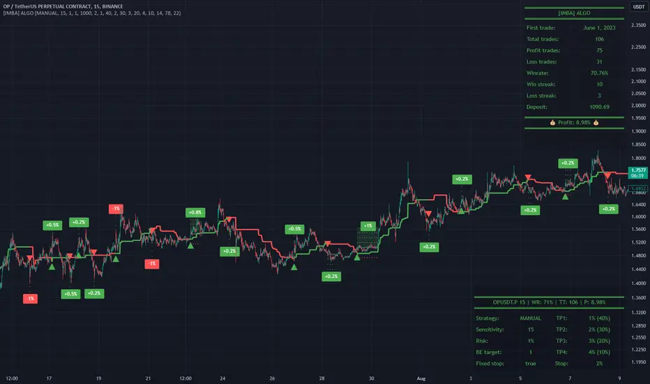
Goldmine Wealth Builder - DKK/SKKGoldmine Wealth Builder
Version 1.0
Introduction to Long-Term Investment Strategies: DKK, SKK1 and SKK2
In the dynamic realm of long-term investing, the DKK, SKK1, and SKK2 strategies stand as valuable pillars. These strategies, meticulously designed to assist investors in building robust portfolios, combine the power of Super Trend, RSI (Relative Strength Index), Exponential Moving Averages (EMAs), and their crossovers. By providing clear alerts and buy signals on a daily time frame, they equip users with the tools needed to make well-informed investment decisions and navigate the complexities of the financial markets. These strategies offer a versatile and structured approach to both conservative and aggressive investment, catering to the diverse preferences and objectives of investors.
Each part of this strategy provides a unique perspective and approach to the accumulation of assets, making it a versatile and comprehensive method for investors seeking to optimize their portfolio performance. By diligently applying this multi-faceted approach, investors can make informed decisions and effectively capitalize on potential market opportunities.
DKK Strategy for ETFs and Funds:
The DKK system is a strategy designed for accumulating ETFs and Funds as long-term investments in your portfolio. It simplifies the process of identifying trend reversals and opportune moments to invest in listed ETFs and Funds, particularly during bull markets. Here's a detailed explanation of the DKK system:
Objective: The primary aim of the DKK system is to build a long-term investment portfolio by focusing on ETFs and Funds. It facilitates the identification of stocks that are in the process of reversing their trends, allowing investors to benefit from upward price movements in these financial instruments.
Stock Selection Criteria: The DKK system employs specific criteria for selecting ETFs and Funds:
• 200EMA (Exponential Moving Average): The system monitors whether the prices of ETFs and Funds are consistently below the 200-day Exponential Moving Average. This is considered an indicator of weakness, especially on a daily time frame.
• RSI (Relative Strength Index): The system looks for an RSI value of less than 40. An RSI below 40 is often seen as an indication of a weak or oversold condition in a financial instrument.
Alert Signal: Once the DKK system identifies ETFs and Funds meeting these criteria, it provides an alert signal:
• Red Upside Triangle Sign: This signal is automatically generated on the daily chart of ETFs and Funds. It serves as a clear indicator to investors that it's an opportune time to accumulate these financial instruments for long-term investment.
It's important to note that the DKK system is specifically designed for ETFs and Funds, so it should be applied to these types of investments. Additionally, it's recommended to track index ETFs and specific types of funds, such as REITs (Real Estate Investment Trusts) and INVITs (Infrastructure Investment Trusts), in line with the DKK system's approach. This strategy simplifies the process of identifying investment opportunities within this asset class, particularly during periods of market weakness.
SKK1 Strategy for Conservative Stock Investment:
The SKK 1 system is a stock investment strategy tailored for conservative investors seeking long-term portfolio growth with a focus on stability and prudent decision-making. This strategy is meticulously designed to identify pivotal market trends and stock price movements, allowing investors to make informed choices and capitalize on upward market trends while minimizing risk. Here's a comprehensive overview of the SKK 1 system, emphasizing its suitability for conservative investors:
Objective: The primary objective of the SKK 1 system is to accumulate stocks as long-term investments in your portfolio while prioritizing capital preservation. It offers a disciplined approach to pinpointing potential entry points for stocks, particularly during market corrections and trend reversals, thereby enabling you to actively participate in bullish market phases while adopting a conservative risk management stance.
Stock Selection Criteria: The SKK 1 system employs a stringent set of criteria to select stocks for investment:
• Correction Mode: It identifies stocks that have undergone a correction, signifying a decline in stock prices from their recent highs. This conservative approach emphasizes the importance of seeking stocks with a history of stability.
• 200EMA (Exponential Moving Average): The system diligently analyses daily stock price movements, specifically looking for stocks that have fallen to or below the 200-day Exponential Moving Average. This indicator suggests potential overselling and aligns with a conservative strategy of buying low.
Trend Reversal Confirmation: The SKK 1 system doesn't merely pinpoint stocks in correction mode; it takes an extra step to confirm a trend reversal. It employs the following indicators:
• Short-term Downtrends Reversal: This aspect focuses on identifying the reversal of short-term downtrends in stock prices, observed through the transition of the super trend indicator from the red zone to the green zone. This cautious approach ensures that the trend is genuinely shifting.
• Super Trend Zones: These zones are crucial for assessing whether a stock is in a bullish or bearish trend. The system consistently monitors these zones to confirm a potential trend reversal.
Alert & Buy Signals: When the SKK 1 system identifies stocks that have reached a potential bottom and are on the verge of a trend reversal, it issues vital alert signals, aiding conservative investors in prudent decision-making:
• Orange Upside Triangle Sign: This signal serves as a cautious heads-up, indicating that a stock may be poised for a trend reversal. It advises investors to prepare funds for potential investment without taking undue risks.
• Green Upside Triangle Sign: This is the confirmation of a trend reversal, signifying a robust buy signal. Conservative investors can confidently enter the market at this point, accumulating stocks for a long-term investment, secure in the knowledge that the trend is in their favor.
In summary, the SKK 1 system is a systematic and conservative approach to stock investing. It excels in identifying stocks experiencing corrections and ensures that investors act when there's a strong indication of a trend reversal, all while prioritizing capital preservation and risk management. This strategy empowers conservative investors to navigate the intricacies of the stock market with confidence, providing a calculated and stable path toward long-term portfolio growth.
Note: The SKK1 strategy, known for its conservative approach to stock investment, also provides an option to extend its methodology to ETFs and Funds for those investors who wish to accumulate assets more aggressively. By enabling this feature in the settings, you can harness the SKK1 strategy's careful criteria and signal indicators to accumulate aggressive investments in ETFs and Funds.
This flexible approach acknowledges that even within a conservative strategy, there may be opportunities for more assertive investments in assets like ETFs and Funds. By making use of this option, you can strike a balance between a conservative stance in your stock portfolio while exploring an aggressive approach in other asset classes. It offers the versatility to cater to a variety of investment preferences, ensuring that you can adapt your strategy to suit your financial goals and risk tolerance.
SKK 2 Strategy for Aggressive Stock Investment:
The SKK 2 strategy is designed for those who are determined not to miss significant opportunities within a continuous uptrend and seek a way to enter a trend that doesn't present entry signals through the SKK 1 strategy. While it offers a more aggressive entry approach, it is ideal for individuals willing to take calculated risks to potentially reap substantial long-term rewards. This strategy is particularly suitable for accumulating stocks for aggressive long-term investment. Here's a detailed description of the SKK 2 strategy:
Objective: The primary aim of the SKK 2 strategy is to provide an avenue for investors to identify short-term trend reversals and seize the opportunity to enter stocks during an uptrend, thereby capitalizing on a sustained bull run. It acknowledges that there may not always be clear entry signals through the SKK 1 strategy and offers a more aggressive alternative.
Stock Selection Criteria: The SKK 2 strategy utilizes a specific set of criteria for stock selection:
1. 50EMA (Exponential Moving Average): It targets stocks that are trading below the 50-day Exponential Moving Average. This signals a short-term reversal from the top and indicates that the stock is in a downtrend.
2. RSI (Relative Strength Index): The strategy considers stocks with an RSI of less than 40, which is an indicator of weakness in the stock.
Alert Signals: The SKK 2 strategy provides distinct alert signals that facilitate entry during an aggressive reversal:
• Red Downside Triangle Sign: This signal is triggered when the stock is below the 50EMA and has an RSI of less than 40. It serves as a clear warning of a short-term reversal from the top and a downtrend, displayed on the daily chart.
• Purple Upside Triangle Sign: This sign is generated when a reversal occurs through a bullish candle, and the RSI is greater than 40. It signifies the stock has bottomed out from a short-term downtrend and is now reversing. This purple upside triangle serves as an entry signal on the chart, presenting an attractive opportunity to accumulate stocks during a strong bullish phase, offering a chance to seize a potentially favorable long-term investment.
In essence, the SKK 2 strategy caters to aggressive investors who are willing to take calculated risks to enter stocks during a continuous uptrend. It focuses on identifying short-term reversals and provides well-defined signals for entry. While this strategy is more aggressive in nature, it has the potential to yield substantial rewards for those who are comfortable with a higher level of risk and are looking for opportunities to build a strong long-term portfolio.
Introduction to Strategy Signal Information Chart
This chart provides essential information on strategy signals for DKK, SKK1, and SKK2. By quickly identifying "Buy" and "Alert" signals for each strategy, investors can efficiently gauge market conditions and make informed decisions to optimize their investment portfolios.
In Conclusion
These investment strategies, whether conservative like DKK and SKK1 or more aggressive like SKK2, offer a range of options for investors to navigate the complex world of long-term investments. The combination of Super Trend, RSI, and EMAs with their crossovers provides clear signals on a daily time frame, empowering users to make well-informed decisions and potentially capitalize on market opportunities. Whether you're looking for stability or are ready to embrace more risk, these strategies have something to offer for building and growing your investment portfolio.

[FN] Strategy - Store Level on ConditionThis is a function that you can use in strategies. Not a strategy in and of itself.
Example thumbnail is showing the function applied to a strategy.
Oftentimes, I am asked a question regarding how to hold a variable at a specific, constant level over a conditional period of time. This question is always asked in a very long convoluted way like "I want the strategy to know what the high of the last pivot was while I'm in a long." or some other variation of wanting a script to remember something from prior bars.
This function is designed to store a price or some numeric level on the bar that your conditional (bool) statements determine that it should be stored. In this construct, you would set conditional statement(s) to flip the 'hold condition' to be true on the next bar, then hold that value until either the "hold condition" is no longer true or the initial conditions trigger again, causing an update to the level that you want to capture.
You still have to come up with the logic for the start condition and hold condition on your own, but I've provided an example that should give you an idea of how to accomplish this and customize/deploy the function for your purposes.
The function will return 'na' when neither the start condition nor hold condition are true. There's multiple ways to implement this and variations on how the level is chosen. I've written extensive notes in the script to guide you through the logic behind the function. My hope is that it will be useful to those trying to build strategies or anyone attempting to get their script to remember a level under given conditions.
In the thumbnail example, the take profit level is defined at the beginning of the trade and held until the take profit order executes. The order execution is a separate matter. However, storing the take-profit level at a static value is key to telling the strategy.exit() function what price to execute a limit exit order at.
Example: strategy.exit("Exit Long", from_entry = "long", qty_percent = 100, limit = stored_value)
Let me know how it works out for you and if I can be of any assistance.
Note: Strategy results are mainly derived from the fact that the strategy is long-only, the NQ only goes up, and there is no stop loss in place. So don't ask for the specific strategy, because unless you're trading a single contract with a $500,000 account, you'll probably get liquidated using this strategy as it is presented.

COT IndexTHE HIDDEN INTELLIGENCE IN FUTURES MARKETS
What if you could see what the smartest players in the futures markets are doing before the crowd catches on? While retail traders chase momentum indicators and moving averages, obsess over Japanese candlestick patterns, and debate whether the RSI should be set to fourteen or twenty-one periods, institutional players leave footprints in the sand through their mandatory reporting to the Commodity Futures Trading Commission. These footprints, published weekly in the Commitment of Traders reports, have been hiding in plain sight for decades, available to anyone with an internet connection, yet remarkably few traders understand how to interpret them correctly. The COT Index indicator transforms this raw institutional positioning data into actionable trading signals, bringing Wall Street intelligence to your trading screen without requiring expensive Bloomberg terminals or insider connections.
The uncomfortable truth is this: Most retail traders operate in a binary world. Long or short. Buy or sell. They apply technical analysis to individual positions, constrained by limited capital that forces them to concentrate risk in single directional bets. Meanwhile, institutional traders operate in an entirely different dimension. They manage portfolios dynamically weighted across multiple markets, adjusting exposure based on evolving market conditions, correlation shifts, and risk assessments that retail traders never see. A hedge fund might be simultaneously long gold, short oil, neutral on copper, and overweight agricultural commodities, with position sizes calibrated to volatility and portfolio Greeks. When they increase gold exposure from five percent to eight percent of portfolio allocation, this rebalancing decision reflects sophisticated analysis of opportunity cost, risk parity, and cross-market dynamics that no individual chart pattern can capture.
This portfolio reweighting activity, multiplied across hundreds of institutional participants, manifests in the aggregate positioning data published weekly by the CFTC. The Commitment of Traders report does not show individual trades or strategies. It shows the collective footprint of how actual commercial hedgers and large speculators have allocated their capital across different markets. When mining companies collectively increase forward gold sales to hedge thirty percent more production than last quarter, they are not reacting to a moving average crossover. They are making strategic allocation decisions based on production forecasts, cost structures, and price expectations derived from operational realities invisible to outside observers. This is portfolio management in action, revealed through positioning data rather than price charts.
If you want to understand how institutional capital actually flows, how sophisticated traders genuinely position themselves across market cycles, the COT report provides a rare window into that hidden world. But understand what you are getting into. This is not a tool for scalpers seeking confirmation of the next five-minute move. This is not an oscillator that flashes oversold at market bottoms with convenient precision. COT analysis operates on a timescale measured in weeks and months, revealing positioning shifts that precede major market turns but offer no precision timing. The data arrives three days stale, published only once per week, capturing strategic positioning rather than tactical entries.
If you need instant gratification, if you trade intraday moves, if you demand mechanical signals with ninety percent accuracy, close this document now. COT analysis rewards patience, position sizing discipline, and tolerance for being early. It punishes impatience, overleveraging, and the expectation that any single indicator can substitute for market understanding.
The premise is deceptively simple. Every Tuesday, large traders in futures markets must report their positions to the CFTC. By Friday afternoon, this data becomes public. Academic research spanning three decades has consistently shown that not all market participants are created equal. Some traders consistently profit while others consistently lose. Some anticipate major turning points while others chase trends into exhaustion. Bessembinder and Chan (1992) demonstrated in their seminal study that commercial hedgers, those with actual exposure to the underlying commodity or financial instrument, possess superior forecasting ability compared to speculators. Their research, published in the Journal of Finance, found statistically significant predictive power in commercial positioning, particularly at extreme levels. This finding challenged the efficient market hypothesis and opened the door to a new approach to market analysis based on positioning rather than price alone.
Think about what this means. Every week, the government publishes a report showing you exactly how the most informed market participants are positioned. Not their opinions. Not their predictions. Their actual money at risk. When agricultural producers collectively hold their largest short hedge in five years, they are not making idle speculation. They are locking in prices for crops they will harvest, informed by private knowledge of weather conditions, soil quality, inventory levels, and demand expectations invisible to outside observers. When energy companies aggressively hedge forward production at current prices, they reveal information about expected supply that no analyst report can capture. This is not technical analysis based on past prices. This is not fundamental analysis based on publicly available data. This is behavioral analysis based on how the smartest money is actually positioned, how institutions allocate capital across portfolios, and how those allocation decisions shift as market conditions evolve.
WHY SOME TRADERS KNOW MORE THAN OTHERS
Building on this foundation, Sanders, Boris and Manfredo (2004) conducted extensive research examining the behaviour patterns of different trader categories. Their work, which analyzed over a decade of COT data across multiple commodity markets, revealed a fascinating dynamic that challenges much of what retail traders are taught. Commercial hedgers consistently positioned themselves against market extremes, buying when speculators were most bearish and selling when speculators reached peak bullishness. The contrarian positioning of commercials was not random noise but rather reflected their superior information about supply and demand fundamentals. Meanwhile, large speculators, primarily hedge funds and commodity trading advisors, exhibited strong trend-following behaviour that often amplified market moves beyond fundamental values. Small traders, the retail participants, consistently entered positions late in trends, frequently near turning points, making them reliable contrary indicators.
Wang (2003) extended this research by demonstrating that the predictive power of commercial positioning varies significantly across different commodity sectors. His analysis of agricultural commodities showed particularly strong forecasting ability, with commercial net positions explaining up to fifteen percent of return variance in subsequent weeks. This finding suggests that the informational advantages of hedgers are most pronounced in markets where physical supply and demand fundamentals dominate, as opposed to purely financial markets where information asymmetries are smaller. When a corn farmer hedges six months of expected harvest, that decision incorporates private observations about rainfall patterns, crop health, pest pressure, and local storage capacity that no distant analyst can match. When an oil refinery hedges crude oil purchases and gasoline sales simultaneously, the spread relationships reveal expectations about refining margins that reflect operational realities invisible in public data.
The theoretical mechanism underlying these empirical patterns relates to information asymmetry and different participant motivations. Commercial hedgers engage in futures markets not for speculative profit but to manage business risks. An agricultural producer selling forward six months of expected harvest is not making a bet on price direction but rather locking in revenue to facilitate financial planning and ensure business viability. However, this hedging activity necessarily incorporates private information about expected supply, inventory levels, weather conditions, and demand trends that the hedger observes through their commercial operations (Irwin and Sanders, 2012). When aggregated across many participants, this private information manifests in collective positioning.
Consider a gold mining company deciding how much forward production to hedge. Management must estimate ore grades, recovery rates, production costs, equipment reliability, labor availability, and dozens of other operational variables that determine whether locking in prices at current levels makes business sense. If the industry collectively hedges more aggressively than usual, it suggests either exceptional production expectations or concern about sustaining current price levels or combination of both. Either way, this positioning reveals information unavailable to speculators analyzing price charts and economic data. The hedger sees the physical reality behind the financial abstraction.
Large speculators operate under entirely different incentives and constraints. Commodity Trading Advisors managing billions in assets typically employ systematic, trend-following strategies that respond to price momentum rather than fundamental supply and demand. When crude oil rallies from sixty dollars to seventy dollars per barrel, these systems generate buy signals. As the rally continues to eighty dollars, position sizes increase. The strategy works brilliantly during sustained trends but becomes a liability at reversals. By the time oil reaches ninety dollars, trend-following funds are maximally long, having accumulated positions progressively throughout the rally. At this point, they represent not smart money anticipating further gains but rather crowded money vulnerable to reversal. Sanders, Boris and Manfredo (2004) documented this pattern across multiple energy markets, showing that extreme speculator positioning typically marked late-stage trend exhaustion rather than early-stage trend development.
Small traders, the retail participants who fall below reporting thresholds, display the weakest forecasting ability. Wang (2003) found that small trader positioning exhibited negative correlation with subsequent returns, meaning their aggregate positioning served as a reliable contrary indicator. The explanation combines several factors. Retail traders often lack the capital reserves to weather normal market volatility, leading to premature exits from positions that would eventually prove profitable. They tend to receive information through slower channels, entering trends after mainstream media coverage when institutional participants are preparing to exit. Perhaps most importantly, they trade with emotion, buying into euphoria and selling into panic at precisely the wrong times.
At major turning points, the three groups often position opposite each other with commercials extremely bearish, large speculators extremely bullish, and small traders piling into longs at the last moment. These high-divergence environments frequently precede increased volatility and trend reversals. The insiders with business exposure quietly exit as the momentum traders hit maximum capacity and retail enthusiasm peaks. Within weeks, the reversal begins, and positions unwind in the opposite sequence.
FROM RAW DATA TO ACTIONABLE SIGNALS
The COT Index indicator operationalizes these academic findings into a practical trading tool accessible through TradingView. At its core, the indicator normalizes net positioning data onto a zero to one hundred scale, creating what we call the COT Index. This normalization is critical because absolute position sizes vary dramatically across different futures contracts and over time. A commercial trader holding fifty thousand contracts net long in crude oil might be extremely bullish by historical standards, or it might be quite neutral depending on the context of total market size and historical ranges. Raw position numbers mean nothing without context. The COT Index solves this problem by calculating where current positioning stands relative to its range over a specified lookback period, typically two hundred fifty-two weeks or approximately five years of weekly data.
The mathematical transformation follows the methodology originally popularized by legendary trader Larry Williams, though the underlying concept appears in statistical normalization techniques across many fields. For any given trader category, we calculate the highest and lowest net position values over the lookback period, establishing the historical range for that specific market and trader group. Current positioning is then expressed as a percentage of this range, where zero represents the most bearish positioning ever seen in the lookback window and one hundred represents the most bullish extreme. A reading of fifty indicates positioning exactly in the middle of the historical range, suggesting neither extreme optimism nor pessimism relative to recent history (Williams and Noseworthy, 2009).
This index-based approach allows for meaningful comparison across different markets and time periods, overcoming the scaling problems inherent in analyzing raw position data. A commercial index reading of eighty-five in gold carries the same interpretive meaning as an eighty-five reading in wheat or crude oil, even though the absolute position sizes differ by orders of magnitude. This standardization enables systematic analysis across entire futures portfolios rather than requiring market-specific expertise for each contract.
The lookback period selection involves a fundamental tradeoff between responsiveness and stability. Shorter lookback periods, perhaps one hundred twenty-six weeks or approximately two and a half years, make the index more sensitive to recent positioning changes. However, it also increases noise and produces more false signals. Longer lookback periods, perhaps five hundred weeks or approximately ten years, create smoother readings that filter short-term noise but become slower to recognize regime changes. The indicator settings allow users to adjust this parameter based on their trading timeframe, risk tolerance, and market characteristics.
UNDERSTANDING CFTC DATA STRUCTURES
The indicator supports both Legacy and Disaggregated COT report formats, reflecting the evolution of CFTC reporting standards over decades of market development. Legacy reports categorize market participants into three broad groups: commercial traders (hedgers with underlying business exposure), non-commercial traders (large speculators seeking profit without commercial interest), and non-reportable traders (small speculators below reporting thresholds). Each category brings distinct motivations and information advantages to the market (CFTC, 2020).
The Disaggregated reports, introduced in September 2009 for physical commodity markets, provide finer granularity by splitting participants into five categories (CFTC, 2009). Producer and merchant positions capture those actually producing, processing, or merchandising the physical commodity. Swap dealers represent financial intermediaries facilitating derivative transactions for clients. Managed money includes commodity trading advisors and hedge funds executing systematic or discretionary strategies. Other reportables encompasses diverse participants not fitting the main categories. Small traders remain as the fifth group, representing retail participation.
This enhanced categorization reveals nuances invisible in Legacy reports, particularly distinguishing between different types of institutional capital and their distinct behavioural patterns. The indicator automatically detects which report type is appropriate for each futures contract and adjusts the display accordingly.
Importantly, Disaggregated reports exist only for physical commodity futures. Agricultural commodities like corn, wheat, and soybeans have Disaggregated reports because clear producer, merchant, and swap dealer categories exist. Energy commodities like crude oil and natural gas similarly have well-defined commercial hedger categories. Metals including gold, silver, and copper also receive Disaggregated treatment (CFTC, 2009). However, financial futures such as equity index futures, Treasury bond futures, and currency futures remain available only in Legacy format. The CFTC has indicated no plans to extend Disaggregated reporting to financial futures due to different market structures and participant categories in these instruments (CFTC, 2020).
THE BEHAVIORAL FOUNDATION
Understanding which trader perspective to follow requires appreciation of their distinct trading styles, success rates, and psychological profiles. Commercial hedgers exhibit anticyclical behaviour rooted in their fundamental knowledge and business imperatives. When agricultural producers hedge forward sales during harvest season, they are not speculating on price direction but rather locking in revenue for crops they will harvest. Their business requires converting volatile commodity exposure into predictable cash flows to facilitate planning and ensure survival through difficult periods. Yet their aggregate positioning reveals valuable information because these hedging decisions incorporate private information about supply conditions, inventory levels, weather observations, and demand expectations that hedgers observe through their commercial operations (Bessembinder and Chan, 1992).
Consider a practical example from energy markets. Major oil companies continuously hedge portions of forward production based on price levels, operational costs, and financial planning needs. When crude oil trades at ninety dollars per barrel, they might aggressively hedge the next twelve months of production, locking in prices that provide comfortable profit margins above their extraction costs. This hedging appears as short positioning in COT reports. If oil rallies further to one hundred dollars, they hedge even more aggressively, viewing these prices as exceptional opportunities to secure revenue. Their short positioning grows increasingly extreme. To an outside observer watching only price charts, the rally suggests bullishness. But the commercial positioning reveals that the actual producers of oil find these prices attractive enough to lock in years of sales, suggesting skepticism about sustaining even higher levels. When the eventual reversal occurs and oil declines back to eighty dollars, the commercials who hedged at ninety and one hundred dollars profit while speculators who chased the rally suffer losses.
Large speculators or managed money traders operate under entirely different incentives and constraints. Their systematic, momentum-driven strategies mean they amplify existing trends rather than anticipate reversals. Trend-following systems, the most common approach among large speculators, by definition require confirmation of trend through price momentum before entering positions (Sanders, Boris and Manfredo, 2004). When crude oil rallies from sixty dollars to eighty dollars per barrel over several months, trend-following algorithms generate buy signals based on moving average crossovers, breakouts, and other momentum indicators. As the rally continues, position sizes increase according to the systematic rules.
However, this approach becomes a liability at turning points. By the time oil reaches ninety dollars after a sustained rally, trend-following funds are maximally long, having accumulated positions progressively throughout the move. At this point, their positioning does not predict continued strength. Rather, it often marks late-stage trend exhaustion. The psychological and mechanical explanation is straightforward. Trend followers by definition chase price momentum, entering positions after trends establish rather than anticipating them. Eventually, they become fully invested just as the trend nears completion, leaving no incremental buying power to sustain the rally. When the first signs of reversal appear, systematic stops trigger, creating a cascade of selling that accelerates the downturn.
Small traders consistently display the weakest track record across academic studies. Wang (2003) found that small trader positioning exhibited negative correlation with subsequent returns in his analysis across multiple commodity markets. This result means that whatever small traders collectively do, the opposite typically proves profitable. The explanation for small trader underperformance combines several factors documented in behavioral finance literature. Retail traders often lack the capital reserves to weather normal market volatility, leading to premature exits from positions that would eventually prove profitable. They tend to receive information through slower channels, learning about commodity trends through mainstream media coverage that arrives after institutional participants have already positioned. Perhaps most importantly, retail traders are more susceptible to emotional decision-making, buying into euphoria and selling into panic at precisely the wrong times (Tharp, 2008).
SETTINGS, THRESHOLDS, AND SIGNAL GENERATION
The practical implementation of the COT Index requires understanding several key features and settings that users can adjust to match their trading style, timeframe, and risk tolerance. The lookback period determines the time window for calculating historical ranges. The default setting of two hundred fifty-two bars represents approximately one year on daily charts or five years on weekly charts, balancing responsiveness with stability. Conservative traders seeking only the most extreme, highest-probability signals might extend the lookback to five hundred bars or more. Aggressive traders seeking earlier entry and willing to accept more false positives might reduce it to one hundred twenty-six bars or even less for shorter-term applications.
The bullish and bearish thresholds define signal generation levels. Default settings of eighty and twenty respectively reflect academic research suggesting meaningful information content at these extremes. Readings above eighty indicate positioning in the top quintile of the historical range, representing genuine extremes rather than temporary fluctuations. Conversely, readings below twenty occupy the bottom quintile, indicating unusually bearish positioning (Briese, 2008).
However, traders must recognize that appropriate thresholds vary by market, trader category, and personal risk tolerance. Some futures markets exhibit wider positioning swings than others due to seasonal patterns, volatility characteristics, or participant behavior. Conservative traders seeking high-probability setups with fewer signals might raise thresholds to eighty-five and fifteen. Aggressive traders willing to accept more false positives for earlier entry could lower them to seventy-five and twenty-five.
The key is maintaining meaningful differentiation between bullish, neutral, and bearish zones. The default settings of eighty and twenty create a clear three-zone structure. Readings from zero to twenty represent bearish territory where the selected trader group holds unusually bearish positions. Readings from twenty to eighty represent neutral territory where positioning falls within normal historical ranges. Readings from eighty to one hundred represent bullish territory where the selected trader group holds unusually bullish positions.
The trading perspective selection determines which participant group the indicator follows, fundamentally shaping interpretation and signal meaning. For counter-trend traders seeking reversal opportunities, monitoring commercial positioning makes intuitive sense based on the academic research discussed earlier. When commercials reach extreme bearish readings below twenty, indicating unprecedented short positioning relative to recent history, they are effectively betting against the crowd. Given their informational advantages demonstrated by Bessembinder and Chan (1992), this contrarian stance often precedes major bottoms.
Trend followers might instead monitor large speculator positioning, but with inverted logic compared to commercials. When managed money reaches extreme bullish readings above eighty, the trend may be exhausting rather than accelerating. This seeming paradox reflects their late-cycle participation documented by Sanders, Boris and Manfredo (2004). Sophisticated traders thus use speculator extremes as fade signals, entering positions opposite to speculator consensus.
Small trader monitoring serves primarily as a contrary indicator for all trading styles. Extreme small trader bullishness above seventy-five or eighty typically warns of retail FOMO at market tops. Extreme small trader bearishness below twenty or twenty-five often marks capitulation bottoms where the last weak hands have sold.
VISUALIZATION AND USER INTERFACE
The visual design incorporates multiple elements working together to facilitate decision-making and maintain situational awareness during active trading. The primary COT Index line plots in bold with adjustable line width, defaulting to two pixels for clear visibility against busy price charts. An optional glow effect, controlled by a simple toggle, adds additional visual prominence through multiple plot layers with progressively increasing transparency and width.
A twenty-one period exponential moving average overlays the index line, providing trend context for positioning changes. When the index crosses above its moving average, it signals accelerating bullish sentiment among the selected trader group regardless of whether absolute positioning is extreme. Conversely, when the index crosses below its moving average, it signals deteriorating sentiment and potentially the beginning of a reversal in positioning trends.
The EMA provides a dynamic reference line for assessing positioning momentum. When the index trades far above its EMA, positioning is not only extreme in absolute terms but also building with momentum. When the index trades far below its EMA, positioning is contracting or reversing, which may indicate weakening conviction even if absolute levels remain elevated.
The data table positioned at the top right of the chart displays eleven metrics for each trader category, transforming the indicator from a simple index calculation into an analytical dashboard providing multidimensional market intelligence. Beyond the COT Index itself, users can monitor positioning extremity, which measures how unusual current levels are compared to historical norms using statistical techniques. The extremity metric clarifies whether a reading represents the ninety-fifth or ninety-ninth percentile, with values above two standard deviations indicating genuinely exceptional positioning.
Market power quantifies each group's influence on total open interest. This metric expresses each trader category's net position as a percentage of total market open interest. A commercial entity holding forty percent of total open interest commands significantly more influence than one holding five percent, making their positioning signals more meaningful.
Momentum and rate of change metrics reveal whether positions are building or contracting, providing early warning of potential regime shifts. Position velocity measures the rate of change in positioning changes, effectively a second derivative providing even earlier insight into inflection points.
Sentiment divergence highlights disagreements between commercial and speculative positioning. This metric calculates the absolute difference between normalized commercial and large speculator index values. Wang (2003) found that these high-divergence environments frequently preceded increased volatility and reversals.
The table also displays concentration metrics when available, showing how positioning is distributed among the largest handful of traders in each category. High concentration indicates a few dominant players controlling most of the positioning, while low concentration suggests broad-based participation across many traders.
THE ALERT SYSTEM AND MONITORING
The alert system, comprising five distinct alert conditions, enables systematic monitoring of dozens of futures markets without constant screen watching. The bullish and bearish COT signal alerts trigger when the index crosses user-defined thresholds, indicating the selected trader group has reached extreme positioning worthy of attention. These alerts fire in real-time as new weekly COT data publishes, typically Friday afternoon following the Tuesday measurement date.
Extreme positioning alerts fire at ninety and ten index levels, representing the top and bottom ten percent of the historical range, warning of particularly stretched readings that historically precede reversals with high probability. When commercials reach a COT Index reading below ten, they are expressing their most bearish stance in the entire lookback period.
The data staleness alert notifies users when COT reports have not updated for more than ten days, preventing reliance on outdated information for trading decisions. Government shutdowns or federal holidays can interrupt the normal Friday publication schedule. Using stale signals while believing them current creates dangerous false confidence.
The indicator's watermark information display positioned in the bottom right corner provides essential context at a glance. This persistent display shows the symbol and timeframe, the COT report date timestamp, days since last update, and the current signal state. A trader analyzing a potential short entry in crude oil can glance at the watermark to instantly confirm positioning context without interrupting analysis flow.
LIMITATIONS AND REALISTIC EXPECTATIONS
Practical application requires understanding both the indicator's considerable strengths and inherent limitations. COT data inherently lags price action by three days, as Tuesday positions are not published until Friday afternoon. This delay means the indicator cannot catch rapid intraday reversals or respond to surprise news events. Traders using the COT Index for timing entries must accept this latency and focus on swing trading and position trading timeframes where three-day lags matter less than in day trading or scalping.
The weekly publication schedule similarly makes the indicator unsuitable for short-term trading strategies requiring immediate feedback. The COT Index works best for traders operating on weekly or longer timeframes, where positioning shifts measured in weeks and months align with trading horizon.
Extreme COT readings can persist far longer than typical technical indicators suggest, testing the patience and capital reserves of traders attempting to fade them. When crude oil enters a sustained bull market driven by genuine supply disruptions, commercial hedgers may maintain bearish positioning for many months as prices grind higher. A commercial COT Index reading of fifteen indicating extreme bearishness might persist for three months while prices continue rallying before finally reversing. Traders without sufficient capital and risk tolerance to weather such drawdowns will exit prematurely, precisely when the signal is about to work (Irwin and Sanders, 2012).
Position sizing discipline becomes paramount when implementing COT-based strategies. Rather than risking large percentages of capital on individual signals, successful COT traders typically allocate modest position sizes across multiple signals, allowing some to take time to mature while others work more quickly.
The indicator also cannot overcome fundamental regime changes that alter the structural drivers of markets. If gold enters a true secular bull market driven by monetary debasement, commercial hedgers may remain persistently bearish as mining companies sell forward years of production at what they perceive as favorable prices. Their positioning indicates valuation concerns from a production cost perspective, but cannot stop prices from rising if investment demand overwhelms physical supply-demand balance.
Similarly, structural changes in market participation can alter the meaning of positioning extremes. The growth of commodity index investing in the two thousands brought massive passive long-only capital into futures markets, fundamentally changing typical positioning ranges. Traders relying on COT signals without recognizing this regime change would have generated numerous false bearish signals during the commodity supercycle from 2003 to 2008.
The research foundation supporting COT analysis derives primarily from commodity markets where the commercial hedger information advantage is most pronounced. Studies specifically examining financial futures like equity indices and bonds show weaker but still present effects. Traders should calibrate expectations accordingly, recognizing that COT analysis likely works better for crude oil, natural gas, corn, and wheat than for the S&P 500, Treasury bonds, or currency futures.
Another important limitation involves the reporting threshold structure. Not all market participants appear in COT data, only those holding positions above specified minimums. In markets dominated by a few large players, concentration metrics become critical for proper interpretation. A single large trader accounting for thirty percent of commercial positioning might skew the entire category if their individual circumstances are idiosyncratic rather than representative.
GOLD FUTURES DURING A HYPOTHETICAL MARKET CYCLE
Consider a practical example using gold futures during a hypothetical but realistic market scenario that illustrates how the COT Index indicator guides trading decisions through a complete market cycle. Suppose gold has rallied from fifteen hundred to nineteen hundred dollars per ounce over six months, driven by inflation concerns following aggressive monetary expansion, geopolitical uncertainty, and sustained buying by Asian central banks for reserve diversification.
Large speculators, operating primarily trend-following strategies, have accumulated increasingly bullish positions throughout this rally. Their COT Index has climbed progressively from forty-five to eighty-five. The table display shows that large speculators now hold net long positions representing thirty-two percent of total open interest, their highest in four years. Momentum indicators show positive readings, indicating positions are still building though at a decelerating rate. Position velocity has turned negative, suggesting the pace of position building is slowing.
Meanwhile, commercial hedgers have responded to the rally by aggressively selling forward production and inventory. Their COT Index has moved inversely to price, declining from fifty-five to twenty. This bearish commercial positioning represents mining companies locking in forward sales at prices they view as attractive relative to production costs. The table shows commercials now hold net short positions representing twenty-nine percent of total open interest, their most bearish stance in five years. Concentration metrics indicate this positioning is broadly distributed across many commercial entities, suggesting the bearish stance reflects collective industry view rather than idiosyncratic positioning by a single firm.
Small traders, attracted by mainstream financial media coverage of gold's impressive rally, have recently piled into long positions. Their COT Index has jumped from forty-five to seventy-eight as retail investors chase the trend. Television financial networks feature frequent segments on gold with bullish guests. Internet forums and social media show surging retail interest. This retail enthusiasm historically marks late-stage trend development rather than early opportunity.
The COT Index indicator, configured to monitor commercial positioning from a contrarian perspective, displays a clear bearish signal given the extreme commercial short positioning. The table displays multiple confirming metrics: positioning extremity shows commercials at the ninety-sixth percentile of bearishness, market power indicates they control twenty-nine percent of open interest, and sentiment divergence registers sixty-five, indicating massive disagreement between commercial hedgers and large speculators. This divergence, the highest in three years, places the market in the historically high-risk category for reversals.
The interpretation requires nuance and consideration of context beyond just COT data. Commercials are not necessarily predicting an imminent crash. Rather, they are hedging business operations at what they collectively view as favorable price levels. However, the data reveals they have sold unusually large quantities of forward production, suggesting either exceptional production expectations for the year ahead or concern about sustaining current price levels or combination of both. Combined with extreme speculator positioning indicating a crowded long trade, and small trader enthusiasm confirming retail FOMO, the confluence suggests elevated reversal risk even if the precise timing remains uncertain.
A prudent trader analyzing this situation might take several actions based on COT Index signals. Existing long positions could be tightened with closer stop losses. Profit-taking on a portion of long exposure could lock in gains while maintaining some participation. Some traders might initiate modest short positions as portfolio hedges, sizing them appropriately for the inherent uncertainty in timing reversals. Others might simply move to the sidelines, avoiding new long entries until positioning normalizes.
The key lesson from case study analysis is that COT signals provide probabilistic edges rather than deterministic predictions. They work over many observations by identifying higher-probability configurations, not by generating perfect calls on individual trades. A fifty-five percent win rate with proper risk management produces substantial profits over time, yet still means forty-five percent of signals will be premature or wrong. Traders must embrace this probabilistic reality rather than seeking the impossible goal of perfect accuracy.
INTEGRATION WITH TRADING SYSTEMS
Integration with existing trading systems represents a natural and powerful use case for COT analysis, adding a positioning dimension to price-based technical approaches or fundamental analytical frameworks. Few traders rely exclusively on a single indicator or methodology. Rather, they build systems that synthesize multiple information sources, with each component addressing different aspects of market behavior.
Trend followers might use COT extremes as regime filters, modifying position sizing or avoiding new trend entries when positioning reaches levels historically associated with reversals. Consider a classic trend-following system based on moving average crossovers and momentum breakouts. Integration of COT analysis adds nuance. When large speculator positioning exceeds ninety or commercial positioning falls below ten, the regime filter recognizes elevated reversal risk. The system might reduce position sizing by fifty percent for new signals during these high-risk periods (Kaufman, 2013).
Mean reversion traders might require COT signal confluence before fading extended moves. When crude oil becomes technically overbought and large speculators show extreme long positioning above eighty-five, both signals confirm. If only technical indicators show extremes while positioning remains neutral, the potential short signal is rejected, avoiding fades of trends with underlying institutional support (Kaufman, 2013).
Discretionary traders can monitor the indicator as a continuous awareness tool, informing bias and position sizing without dictating mechanical entries and exits. A discretionary trader might notice commercial positioning shifting from neutral to progressively more bullish over several months. This trend informs growing positive bias even without triggering mechanical signals.
Multi-timeframe analysis represents another powerful integration approach. A trader might use daily charts for trade execution and timing while monitoring weekly COT positioning for strategic context. When both timeframes align, highest-probability opportunities emerge.
Portfolio construction for futures traders can incorporate COT signals as an additional selection criterion. Markets showing strong technical setups AND favorable COT positioning receive highest allocations. Markets with strong technicals but neutral or unfavorable positioning receive reduced allocations.
ADVANCED METRICS AND INTERPRETATION
The metrics table transforms simple positioning data into multidimensional market intelligence. Position extremity, calculated as the absolute deviation from the historical mean normalized by standard deviation, helps identify truly unusual readings versus routine fluctuations. A reading above two standard deviations indicates ninety-fifth percentile or higher extremity. Above three standard deviations indicates ninety-ninth percentile or higher, genuinely rare positioning that historically precedes major events with high probability.
Market power, expressed as a percentage of total open interest, reveals whose positioning matters most from a mechanical market impact perspective. Consider two scenarios in gold futures. In scenario one, commercials show a COT Index reading of fifteen while their market power metric shows they hold net shorts representing thirty-five percent of open interest. This is a high-confidence bearish signal. In scenario two, commercials also show a reading of fifteen, but market power shows only eight percent. While positioning is extreme relative to this category's normal range, their limited market share means less mechanical influence on price.
The rate of change and momentum metrics highlight whether positions are accelerating or decelerating, often providing earlier warnings than absolute levels alone. A COT Index reading of seventy-five with rapidly building momentum suggests continued movement toward extremes. Conversely, a reading of eighty-five with decelerating or negative momentum indicates the positioning trend is exhausting.
Position velocity measures the rate of change in positioning changes, effectively a second derivative. When velocity shifts from positive to negative, it indicates that while positioning may still be growing, the pace of growth is slowing. This deceleration often precedes actual reversal in positioning direction by several weeks.
Sentiment divergence calculates the absolute difference between normalized commercial and large speculator index values. When commercials show extreme bearish positioning at twenty while large speculators show extreme bullish positioning at eighty, the divergence reaches sixty, representing near-maximum disagreement. Wang (2003) found that these high-divergence environments frequently preceded increased volatility and reversals. The mechanism is intuitive. Extreme divergence indicates the informed hedgers and momentum-following speculators have positioned opposite each other with conviction. One group will prove correct and profit while the other proves incorrect and suffers losses. The resolution of this disagreement through price movement often involves volatility.
The table also displays concentration metrics when available. High concentration indicates a few dominant players controlling most of the positioning within a category, while low concentration suggests broad-based participation. Broad-based positioning more reliably reflects collective market intelligence and industry consensus. If mining companies globally all independently decide to hedge aggressively at similar price levels, it suggests genuine industry-wide view about price valuations rather than circumstances specific to one firm.
DATA QUALITY AND RELIABILITY
The CFTC has maintained COT reporting in various forms since the nineteen twenties, providing nearly a century of positioning data across multiple market cycles. However, data quality and reporting standards have evolved substantially over this long period. Modern electronic reporting implemented in the late nineteen nineties and early two thousands significantly improved accuracy and timeliness compared to earlier paper-based systems.
Traders should understand that COT reports capture positions as of Tuesday's close each week. Markets remain open three additional days before publication on Friday afternoon, meaning the reported data is three days stale when received. During periods of rapid market movement or major news events, this lag can be significant. The indicator addresses this limitation by including timestamp information and staleness warnings.
The three-day lag creates particular challenges during extreme volatility episodes. Flash crashes, surprise central bank interventions, geopolitical shocks, and other high-impact events can completely transform market positioning within hours. Traders must exercise judgment about whether reported positioning remains relevant given intervening events.
Reporting thresholds also mean that not all market participants appear in disaggregated COT data. Traders holding positions below specified minimums aggregate into the non-reportable or small trader category. This aggregation affects different markets differently. In highly liquid contracts like crude oil with thousands of participants, reportable traders might represent seventy to eighty percent of open interest. In thinly traded contracts with only dozens of active participants, a few large reportable positions might represent ninety-five percent of open interest.
Another data quality consideration involves trader classification into categories. The CFTC assigns traders to commercial or non-commercial categories based on reported business purpose and activities. However, this process is not perfect. Some entities engage in both commercial and speculative activities, creating ambiguity about proper classification. The transition to Disaggregated reports attempted to address some of these ambiguities by creating more granular categories.
COMPARISON WITH ALTERNATIVE APPROACHES
Several alternative approaches to COT analysis exist in the trading community beyond the normalization methodology employed by this indicator. Some analysts focus on absolute position changes week-over-week rather than index-based normalization. This approach calculates the change in net positioning from one week to the next. The emphasis falls on momentum in positioning changes rather than absolute levels relative to history. This method potentially identifies regime shifts earlier but sacrifices cross-market comparability (Briese, 2008).
Other practitioners employ more complex statistical transformations including percentile rankings, z-score standardization, and machine learning classification algorithms. Ruan and Zhang (2018) demonstrated that machine learning models applied to COT data could achieve modest improvements in forecasting accuracy compared to simple threshold-based approaches. However, these gains came at the cost of interpretability and implementation complexity.
The COT Index indicator intentionally employs a relatively straightforward normalization methodology for several important reasons. First, transparency enhances user understanding and trust. Traders can verify calculations manually and develop intuitive feel for what different readings mean. Second, academic research suggests that most of the predictive power in COT data comes from extreme positioning levels rather than subtle patterns requiring complex statistical methods to detect. Third, robust methods that work consistently across many markets and time periods tend to be simpler rather than more complex, reducing the risk of overfitting to historical data. Fourth, the complexity costs of implementation matter for retail traders without programming teams or computational infrastructure.
PSYCHOLOGICAL ASPECTS OF COT TRADING
Trading based on COT data requires psychological fortitude that differs from momentum-based approaches. Contrarian positioning signals inherently mean betting against prevailing market sentiment and recent price action. When commercials reach extreme bearish positioning, prices have typically been rising, sometimes for extended periods. The price chart looks bullish, momentum indicators confirm strength, moving averages align positively. The COT signal says bet against all of this. This psychological difficulty explains why COT analysis remains underutilized relative to trend-following methods.
Human psychology strongly predisposes us toward extrapolation and recency bias. When prices rally for months, our pattern-matching brains naturally expect continued rally. The recent price action dominates our perception, overwhelming rational analysis about positioning extremes and historical probabilities. The COT signal asking us to sell requires overriding these powerful psychological impulses.
The indicator design attempts to support the required psychological discipline through several features. Clear threshold markers and signal states reduce ambiguity about when signals trigger. When the commercial index crosses below twenty, the signal is explicit and unambiguous. The background shifts to red, the signal label displays bearish, and alerts fire. This explicitness helps traders act on signals rather than waiting for additional confirmation that may never arrive.
The metrics table provides analytical justification for contrarian positions, helping traders maintain conviction during inevitable periods of adverse price movement. When a trader enters short positions based on extreme commercial bearish positioning but prices continue rallying for several weeks, doubt naturally emerges. The table display provides reassurance. Commercial positioning remains extremely bearish. Divergence remains high. The positioning thesis remains intact even though price action has not yet confirmed.
Alert functionality ensures traders do not miss signals due to inattention while also not requiring constant monitoring that can lead to emotional decision-making. Setting alerts for COT extremes enables a healthier relationship with markets. When meaningful signals occur, alerts notify them. They can then calmly assess the situation and execute planned responses.
However, no indicator design can completely overcome the psychological difficulty of contrarian trading. Some traders simply cannot maintain short positions while prices rally. For these traders, COT analysis might be better employed as an exit signal for long positions rather than an entry signal for shorts.
Ultimately, successful COT trading requires developing comfort with probabilistic thinking rather than certainty-seeking. The signals work over many observations by identifying higher-probability configurations, not by generating perfect calls on individual trades. A fifty-five or sixty percent win rate with proper risk management produces substantial profits over years, yet still means forty to forty-five percent of signals will be premature or wrong. COT analysis provides genuine edge, but edge means probability advantage, not elimination of losing trades.
EDUCATIONAL RESOURCES AND CONTINUOUS LEARNING
The indicator provides extensive built-in educational resources through its documentation, detailed tooltips, and transparent calculations. However, mastering COT analysis requires study beyond any single tool or resource. Several excellent resources provide valuable extensions of the concepts covered in this guide.
Books and practitioner-focused monographs offer accessible entry points. Stephen Briese published The Commitments of Traders Bible in two thousand eight, offering detailed breakdowns of how different markets and trader categories behave (Briese, 2008). Briese's work stands out for its empirical focus and market-specific insights. Jack Schwager includes discussion of COT analysis within the broader context of market behavior in his book Market Sense and Nonsense (Schwager, 2012). Perry Kaufman's Trading Systems and Methods represents perhaps the most rigorous practitioner-focused text on systematic trading approaches including COT analysis (Kaufman, 2013).
Academic journal articles provide the rigorous statistical foundation underlying COT analysis. The Journal of Futures Markets regularly publishes research on positioning data and its predictive properties. Bessembinder and Chan's earlier work on systematic risk, hedging pressure, and risk premiums in futures markets provides theoretical foundation (Bessembinder, 1992). Chang's examination of speculator returns provides historical context (Chang, 1985). Irwin and Sanders provide essential skeptical perspective in their two thousand twelve article (Irwin and Sanders, 2012). Wang's two thousand three article provides one of the most empirical analyses of COT data across multiple commodity markets (Wang, 2003).
Online resources extend beyond academic and book-length treatments. The CFTC website provides free access to current and historical COT reports in multiple formats. The explanatory materials section offers detailed documentation of report construction, category definitions, and historical methodology changes. Traders serious about COT analysis should read these official CFTC documents to understand exactly what they are analyzing.
Commercial COT data services such as Barchart provide enhanced visualization and analysis tools beyond raw CFTC data. TradingView's educational materials, published scripts library, and user community provide additional resources for exploring different approaches to COT analysis.
The key to mastering COT analysis lies not in finding a single definitive source but rather in building understanding through multiple perspectives and information sources. Academic research provides rigorous empirical foundation. Practitioner-focused books offer practical implementation insights. Direct engagement with data through systematic backtesting develops intuition about how positioning dynamics manifest across different market conditions.
SYNTHESIZING KNOWLEDGE INTO PRACTICE
The COT Index indicator represents the synthesis of academic research, trading experience, and software engineering into a practical tool accessible to retail traders equipped with nothing more than a TradingView account and willingness to learn. What once required expensive data subscriptions, custom programming capabilities, statistical software, and institutional resources now appears as a straightforward indicator requiring only basic parameter selection and modest study to understand. This democratization of institutional-grade analysis tools represents a broader trend in financial markets over recent decades.
Yet technology and data access alone provide no edge without understanding and discipline. Markets remain relentlessly efficient at eliminating edges that become too widely known and mechanically exploited. The COT Index indicator succeeds only when users invest time learning the underlying concepts, understand the limitations and probability distributions involved, and integrate signals thoughtfully into trading plans rather than applying them mechanically.
The academic research demonstrates conclusively that institutional positioning contains genuine information about future price movements, particularly at extremes where commercial hedgers are maximally bearish or bullish relative to historical norms. This informational content is neither perfect nor deterministic but rather probabilistic, providing edge over many observations through identification of higher-probability configurations. Bessembinder and Chan's finding that commercial positioning explained modest but significant variance in future returns illustrates this probabilistic nature perfectly (Bessembinder and Chan, 1992). The effect is real and statistically significant, yet it explains perhaps ten to fifteen percent of return variance rather than most variance. Much of price movement remains unpredictable even with positioning intelligence.
The practical implication is that COT analysis works best as one component of a trading system rather than a standalone oracle. It provides the positioning dimension, revealing where the smart money has positioned and where the crowd has followed, but price action analysis provides the timing dimension. Fundamental analysis provides the catalyst dimension. Risk management provides the survival dimension. These components work together synergistically.
The indicator's design philosophy prioritizes transparency and education over black-box complexity, empowering traders to understand exactly what they are analyzing and why. Every calculation is documented and user-adjustable. The threshold markers, background coloring, tables, and clear signal states provide multiple reinforcing channels for conveying the same information.
This educational approach reflects a conviction that sustainable trading success comes from genuine understanding rather than mechanical system-following. Traders who understand why commercial positioning matters, how different trader categories behave, what positioning extremes signify, and where signals fit within probability distributions can adapt when market conditions change. Traders mechanically following black-box signals without comprehension abandon systems after normal losing streaks.
The research foundation supporting COT analysis comes primarily from commodity markets where commercial hedger informational advantages are most pronounced. Agricultural producers hedging crops know more about supply conditions than distant speculators. Energy companies hedging production know more about operating costs than financial traders. Metals miners hedging output know more about ore grades than index funds. Financial futures markets show weaker but still present effects.
The journey from reading this documentation to profitable trading based on COT analysis involves several stages that cannot be rushed. Initial reading and basic understanding represents the first stage. Historical study represents the second stage, reviewing past market cycles to observe how positioning extremes preceded major turning points. Paper trading or small-size real trading represents the third stage to experience the psychological challenges. Refinement based on results and personal psychology represents the fourth stage.
Markets will continue evolving. New participant categories will emerge. Regulatory structures will change. Technology will advance. Yet the fundamental dynamics driving COT analysis, that different market participants have different information, different motivations, and different forecasting abilities that manifest in their positioning, will persist as long as futures markets exist. While specific thresholds or optimal parameters may shift over time, the core logic remains sound and adaptable.
The trader equipped with this indicator, understanding of the theory and evidence behind COT analysis, realistic expectations about probability rather than certainty, discipline to maintain positions through adverse volatility, and patience to allow signals time to develop possesses genuine edge in markets. The edge is not enormous, markets cannot allow large persistent inefficiencies without arbitraging them away, but it is real, measurable, and exploitable by those willing to invest in learning and disciplined application.
REFERENCES
Bessembinder, H. (1992) Systematic risk, hedging pressure, and risk premiums in futures markets, Review of Financial Studies, 5(4), pp. 637-667.
Bessembinder, H. and Chan, K. (1992) The profitability of technical trading rules in the Asian stock markets, Pacific-Basin Finance Journal, 3(2-3), pp. 257-284.
Briese, S. (2008) The Commitments of Traders Bible: How to Profit from Insider Market Intelligence. Hoboken: John Wiley & Sons.
Chang, E.C. (1985) Returns to speculators and the theory of normal backwardation, Journal of Finance, 40(1), pp. 193-208.
Commodity Futures Trading Commission (CFTC) (2009) Explanatory Notes: Disaggregated Commitments of Traders Report. Available at: www.cftc.gov (Accessed: 15 January 2025).
Commodity Futures Trading Commission (CFTC) (2020) Commitments of Traders: About the Report. Available at: www.cftc.gov (Accessed: 15 January 2025).
Irwin, S.H. and Sanders, D.R. (2012) Testing the Masters Hypothesis in commodity futures markets, Energy Economics, 34(1), pp. 256-269.
Kaufman, P.J. (2013) Trading Systems and Methods. 5th edn. Hoboken: John Wiley & Sons.
Ruan, Y. and Zhang, Y. (2018) Forecasting commodity futures prices using machine learning: Evidence from the Chinese commodity futures market, Applied Economics Letters, 25(12), pp. 845-849.
Sanders, D.R., Boris, K. and Manfredo, M. (2004) Hedgers, funds, and small speculators in the energy futures markets: an analysis of the CFTC's Commitments of Traders reports, Energy Economics, 26(3), pp. 425-445.
Schwager, J.D. (2012) Market Sense and Nonsense: How the Markets Really Work and How They Don't. Hoboken: John Wiley & Sons.
Tharp, V.K. (2008) Super Trader: Make Consistent Profits in Good and Bad Markets. New York: McGraw-Hill.
Wang, C. (2003) The behavior and performance of major types of futures traders, Journal of Futures Markets, 23(1), pp. 1-31.
Williams, L.R. and Noseworthy, M. (2009) The Right Stock at the Right Time: Prospering in the Coming Good Years. Hoboken: John Wiley & Sons.
FURTHER READING
For traders seeking to deepen their understanding of COT analysis and futures market positioning beyond this documentation, the following resources provide valuable extensions:
Academic Journal Articles:
Fishe, R.P.H. and Smith, A. (2012) Do speculators drive commodity prices away from supply and demand fundamentals?, Journal of Commodity Markets, 1(1), pp. 1-16.
Haigh, M.S., Hranaiova, J. and Overdahl, J.A. (2007) Hedge funds, volatility, and liquidity provision in energy futures markets, Journal of Alternative Investments, 9(4), pp. 10-38.
Kocagil, A.E. (1997) Does futures speculation stabilize spot prices? Evidence from metals markets, Applied Financial Economics, 7(1), pp. 115-125.
Sanders, D.R. and Irwin, S.H. (2011) The impact of index funds in commodity futures markets: A systems approach, Journal of Alternative Investments, 14(1), pp. 40-49.
Books and Practitioner Resources:
Murphy, J.J. (1999) Technical Analysis of the Financial Markets: A Guide to Trading Methods and Applications. New York: New York Institute of Finance.
Pring, M.J. (2002) Technical Analysis Explained: The Investor's Guide to Spotting Investment Trends and Turning Points. 4th edn. New York: McGraw-Hill.
Federal Reserve and Research Institution Publications:
Federal Reserve Banks regularly publish working papers examining commodity markets, futures positioning, and price discovery mechanisms. The Federal Reserve Bank of San Francisco and Federal Reserve Bank of Kansas City maintain active research programs in this area.
Online Resources:
The CFTC website provides free access to current and historical COT reports, explanatory materials, and regulatory documentation.
Barchart offers enhanced COT data visualization and screening tools.
TradingView's community library contains numerous published scripts and educational materials exploring different approaches to positioning analysis.

Silver Bullet ICT Strategy [TradingFinder] 10-11 AM NY Time +FVG🔵 Introduction
The ICT Silver Bullet trading strategy is a precise, time-based algorithmic approach that relies on Fair Value Gaps and Liquidity to identify high-probability trade setups. The strategy primarily focuses on the New York AM Session from 10:00 AM to 11:00 AM, leveraging heightened market activity within this critical window to capture short-term trading opportunities.
As an intraday strategy, it is most effective on lower timeframes, with ICT recommending a 15-minute chart or lower. While experienced traders often utilize 1-minute to 5-minute charts, beginners may find the 1-minute timeframe more manageable for applying this strategy.
This approach specifically targets quick trades, designed to take advantage of market movements within tight one-hour windows. By narrowing its focus, the Silver Bullet offers a streamlined and efficient method for traders to capitalize on liquidity shifts and price imbalances with precision.
In the fast-paced world of forex trading, the ability to identify market manipulation and false price movements is crucial for traders aiming to stay ahead of the curve. The Silver Bullet Indicator simplifies this process by integrating ICT principles such as liquidity traps, Order Blocks, and Fair Value Gaps (FVG).
These concepts form the foundation of a tool designed to mimic the strategies of institutional players, empowering traders to align their trades with the "smart money." By transforming complex market dynamics into actionable insights, the Silver Bullet Indicator provides a powerful framework for short-term trading success
Silver Bullet Bullish Setup :
Silver Bullet Bearish Setup :
🔵 How to Use
The Silver Bullet Indicator is a specialized tool that operates within the critical time windows of 9:00-10:00 and 10:00-11:00 in the forex market. Its design incorporates key principles from ICT (Inner Circle Trader) methodology, focusing on concepts such as liquidity traps, CISD Levels, Order Blocks, and Fair Value Gaps (FVG) to provide precise and actionable trade setups.
🟣 Bullish Setup
In a bullish setup, the indicator starts by marking the high and low of the session, serving as critical reference points for liquidity. A typical sequence involves a liquidity grab below the low, where the price manipulates retail traders into selling positions by breaching a key support level.
This movement is often orchestrated by smart money to accumulate buy orders. Following this liquidity grab, a market structure shift (MSS) occurs, signaled by the price breaking the CISD Level—a confirmation of bullish intent. The indicator then highlights an Order Block near the CISD Level, representing the zone where institutional buying is concentrated.
Additionally, it identifies a Fair Value Gap, which acts as a high-probability area for price retracement and trade entry. Traders can confidently take long positions when the price revisits these zones, targeting the next significant liquidity pool or resistance level.
Bullish Setup in CAPITALCOM:US100 :
🟣 Bearish Setup
Conversely, in a bearish setup, the price manipulates liquidity by creating a false breakout above the high of the session. This move entices retail traders into long positions, allowing institutional players to enter sell orders.
Once the price reverses direction and breaches the CISD Level to the downside, a change of character (CHOCH) becomes evident, confirming a bearish market structure. The indicator highlights an Order Block near this level, indicating the origin of the institutional sell orders, along with an associated FVG, which represents an imbalance zone likely to be revisited before the price continues downward.
By entering short positions when the price retraces to these levels, traders align their strategies with the anticipated continuation of bearish momentum, targeting nearby liquidity voids or support zones.
Bearish Setup in OANDA:XAUUSD :
🔵 Settings
Refine Order Block : Enables finer adjustments to Order Block levels for more accurate price responses.
Mitigation Level OB : Allows users to set specific reaction points within an Order Block, including: Proximal: Closest level to the current price. 50% OB: Midpoint of the Order Block. Distal: Farthest level from the current price.
FVG Filter : The Judas Swing indicator includes a filter for Fair Value Gap (FVG), allowing different filtering based on FVG width: FVG Filter Type: Can be set to "Very Aggressive," "Aggressive," "Defensive," or "Very Defensive." Higher defensiveness narrows the FVG width, focusing on narrower gaps.
Mitigation Level FVG : Like the Order Block, you can set price reaction levels for FVG with options such as Proximal, 50% OB, and Distal.
CISD : The Bar Back Check option enables traders to specify the number of past candles checked for identifying the CISD Level, enhancing CISD Level accuracy on the chart.
🔵 Conclusion
The Silver Bullet Indicator is a cutting-edge tool designed specifically for forex traders who aim to leverage market dynamics during critical liquidity windows. By focusing on the highly active 9:00-10:00 and 10:00-11:00 timeframes, the indicator simplifies complex market concepts such as liquidity traps, Order Blocks, Fair Value Gaps (FVG), and CISD Levels, transforming them into actionable insights.
What sets the Silver Bullet Indicator apart is its precision in detecting false breakouts and market structure shifts (MSS), enabling traders to align their strategies with institutional activity. The visual clarity of its signals, including color-coded zones and directional arrows, ensures that both novice and experienced traders can easily interpret and apply its findings in real-time.
By integrating ICT principles, the indicator empowers traders to identify high-probability entry and exit points, minimize risk, and optimize trade execution. Whether you are capturing short-term price movements or navigating complex market conditions, the Silver Bullet Indicator offers a robust framework to enhance your trading performance.
Ultimately, this tool is more than just an indicator; it is a strategic ally for traders who seek to decode the movements of smart money and capitalize on institutional strategies. With the Silver Bullet Indicator, traders can approach the market with greater confidence, precision, and profitability.

RSI Missmatch(Divergence) OSC. by Neo_ with Missmatch Alert█ Definition
A divergence or missmatch occurs when an asset’s price is moving opposite to a specific technical indicator or is moving in a different direction from other relevant data. The divergence indicator warns traders and technical analysts of changes in a price trend, oftentimes that it is weakening or changing direction.
Divergence or missmatch can be either positive, signifying the possibility of a move that is higher in the asset’s price, or it can be negative, signifying the possibility of a move that is lower in the asset’s price.
█ Takeaways
Divergence or missmatch often works with other indicators and data. It is usually used by technical analysts and traders when the asset’s price is moving counter to the direction of another indicator.
As mentioned above, positive divergence or missmatch indicates that the price could start rising and usually occurs when the price is moving lower, but while another indicator counters this direction by moving higher. In other words, showing bullish signals.
Negative divergence or missmatch indicates that the price could start declining and usually occurs when the price is moving higher, while another indicator moves lower as well. In other words, showing bearish signals.
█ What to look for
Divergence or missmatch is most often used to track and analyze the momentum in an asset’s price and the odds of a price reversal within the current trend. While using divergence, traders and analysts can decide on whether or not they would like to exit the position or set a stop loss in the case the divergence is negative and prices begin to fall.
█ Limitations
It is best to use divergence or missmatch with the aid of other indicators and analysis tools in order to help identify and confirm trend reversals and major market patterns. Divergence should not be relied on by itself to tell you the pertinent information you need to know as an investor. Risk control is key in your analysis and the fact that divergence is not always present in price reversals should definitely be what pushes you to combine it with other tools and indicators.
Additionally, divergence or missmatch can reflect long-term or short-term changes. When making snap decisions, acting on divergence alone could prove detrimental to your trading. Make sure you have other risk factors applied to your charting and general market analysis.
█ What exactly is RSI Missmatches discrepancies using a lookback period in trading?
In trading, lookback period is the number of periods of historical data used for observation and calculation. It is how far into the past the system looks when trying to calculate the variable under consideration. The concept was based on the fact that history can provide information about the future, and my aim was to predict the periods when trend changes would begin within these periods with the RSI oscillator. But this is only true if you're locked back far enough, not locked any further or less!
We already use the idea of looking back in different aspects of our lives, and even in the world of financial trading it can be used in various ways. Of course you will want to learn more about the concept, so in this article we will cover the following topics:
█ What kind of hindsight is this?
The aim here is to check whether trends will change in certain cycles, so we chose the High + Low / 2 formula as the source. Because no matter how much the prices swing up or down, sometimes the rebound can go further. The aim here is to notice the points where the price leaves a needle at the levels where it oscillates and the slowdown in momentum.
█ What does look-back period mean in trade?
To understand what a lookback period means in trading, you need to ask yourself: What is a lookback period in trading? In financial trading, period refers to the duration of a particular trading session. For example, a one-week period means one full week of trading sessions or five trading days. In 5 trading days, the average time is 120 hours in FX markets and 40 hours in stock markets. Regardless of what happens in these cycles, I prefer to choose a time period of 55 periods. Because I noticed that in all the charts I examined, the cycles generally changed during this time period.
█ Let's talk about the meaning of catching Missmatches
As you know, technical indicators are all a mathematical calculation using historical market data (price, volume, or a combination of both). It shows the behavior of the price better and helps in the analysis of price movement. But the indicator can only serve your intended purpose if you get the lookback time right. What we mean here is the setting parameter that determines how much historical data it will use in its calculation. In other words, it is the retrospective review period.
For example, on the RSI indicator you can set this period to 13 periods (default setting) or even 2 periods. The period you choose can determine what the indicator tells you, which in turn determines the strategy you can create with the indicator. The 13- period RSI gives you information about price momentum, so you can effectively use it to create a momentum strategy. On the other hand, the 2-periods RSI can be used to create a mean reversion strategy. To catch any incompatibilities, I set this period to 55 periods. Nothing more, nothing less!
█ Summary
The missmatch indicator helps traders assess changes in the price trend and indicates when price will move with or against the direction of another indicator. It can be either positive or negative, but it is important to note its limitations and that it should be used with other indicators that can also monitor price trends.
We wish you to identify these incompatibilities in the market in the best way possible... Good luck.
█ Tanım
Bir varlığın fiyatı belirli bir teknik göstergenin tersi yönünde hareket ettiğinde veya diğer ilgili verilerden farklı bir yönde hareket ettiğinde bir sapma veya uyumsuzluk meydana gelir. Farklılık göstergesi, tüccarları ve teknik analistleri fiyat eğilimindeki değişiklikler konusunda uyarır; çoğu zaman zayıflıyor veya yön değiştiriyor.
Farklılık veya uyumsuzluk, varlığın fiyatında daha yüksek bir hareket olasılığını işaret ederek pozitif olabilir veya varlığın fiyatında daha düşük bir hareket olasılığını işaret ederek negatif olabilir.
█ Çıkarımlar
Farklılık veya uyumsuzluk çoğu zaman diğer göstergeler ve verilerle de çalışır. Genellikle teknik analistler ve yatırımcılar tarafından varlığın fiyatı başka bir göstergenin yönünün tersine hareket ettiğinde kullanılır.
Yukarıda bahsedildiği gibi pozitif sapma veya uyumsuzluk, fiyatın yükselmeye başlayabileceğini gösterir ve genellikle fiyat düşerken meydana gelir, ancak başka bir gösterge bu yöne yükselerek karşı koyar. Başka bir deyişle yükseliş sinyalleri veriyor.
Negatif sapma veya uyumsuzluk, fiyatın düşmeye başlayabileceğini gösterir ve genellikle fiyat yükselirken başka bir gösterge de düşerken meydana gelir. Başka bir deyişle düşüş sinyalleri veriyor.
█ Nelere bakılmalı
Farklılık veya uyumsuzluk çoğunlukla bir varlığın fiyatındaki momentumu ve mevcut trend içinde fiyatın tersine dönme olasılığını izlemek ve analiz etmek için kullanılır. Farklılaşmayı kullanırken tüccarlar ve analistler, sapmanın negatif olması ve fiyatların düşmeye başlaması durumunda pozisyondan çıkmak isteyip istemeyeceklerine veya zararı durdurma kararı verip veremeyeceklerine karar verebilirler.
█ Sınırlamalar
Trend dönüşlerini ve ana piyasa modellerini tanımlamaya ve doğrulamaya yardımcı olmak için diğer göstergeler ve analiz araçlarının yardımıyla sapmayı veya uyumsuzluğu kullanmak en iyisidir. Bir yatırımcı olarak bilmeniz gereken ilgili bilgileri size söylemesi için farklılığa tek başına güvenilmemelidir. Risk kontrolü analizinizin anahtarıdır ve fiyat dönüşlerinde farklılığın her zaman mevcut olmaması gerçeği kesinlikle sizi onu diğer araç ve göstergelerle birleştirmeye iten şey olmalıdır.
Ek olarak, farklılık veya uyumsuzluk uzun vadeli veya kısa vadeli değişiklikleri yansıtabilir. Ani kararlar verirken yalnızca farklılıklara göre hareket etmek ticaretinize zarar verebilir. Grafiğinize ve genel piyasa analizinize başka risk faktörlerinin uygulandığından emin olun.
█ Ticarette yeniden inceleme dönemi kullanan RSI Missmatches tutarsızlıkları tam olarak nedir?
Ticarette yeniden inceleme süresi, gözlem ve hesaplama için kullanılan geçmiş verilerin dönemlerinin sayısıdır. Söz konusu değişkeni hesaplamaya çalışırken sistemin ne kadar geçmişe baktığıdır. Konsept tarihin geleceğe dair bilgi verebileceği gerçeği üzerine kuruluydu ve amacım RSI osilatörü ile bu dönemler içerisinde trend değişimlerinin başlayacağı dönemleri tahmin etmekti. Ancak bu yalnızca yeterince geriye kilitlenmişseniz geçerlidir, daha fazla veya daha az kilitlenmemişseniz!
Geriye bakma fikrini hayatımızın farklı yönlerinde zaten kullanıyoruz ve hatta finansal ticaret dünyasında bile bu fikir çeşitli şekillerde kullanılabilir. Elbette konsept hakkında daha fazla bilgi edinmek isteyeceksiniz, bu nedenle bu yazıda aşağıdaki konuları ele alacağız:
█ Bu nasıl bir sonradan görmedir?
Burada amaç belli döngülerde trendlerin değişip değişmeyeceğini kontrol etmek olduğundan kaynak olarak Yüksek + Düşük / 2 formülünü seçtik. Çünkü fiyatlar ne kadar yukarı veya aşağı hareket ederse etsin bazen toparlanma daha da ileri gidebiliyor. Burada amaç fiyatın salınım yaptığı seviyelerde iğne bıraktığı noktaları ve momentumdaki yavaşlamayı fark etmektir.
█ Ticarette geriye bakma süresi ne anlama geliyor?
Ticarette yeniden inceleme süresinin ne anlama geldiğini anlamak için kendinize şu soruyu sormanız gerekir: Ticarette yeniden inceleme süresi nedir? Finansal ticarette dönem, belirli bir ticaret seansının süresini ifade eder. Örneğin, bir haftalık dönem, bir tam haftalık işlem seansı veya beş işlem günü anlamına gelir. 5 işlem gününde ortalama süre döviz piyasalarında 120 saat, borsalarda ise 40 saattir. Bu döngülerde ne olursa olsun 55 periyotluk bir zaman dilimini seçmeyi tercih ediyorum. Çünkü incelediğim tüm grafiklerde bu zaman diliminde döngülerin genel olarak değiştiğini fark ettim.
█ Kaçak Eşleşmeleri yakalamanın anlamı hakkında konuşalım
Bildiğiniz gibi teknik göstergeler, geçmiş piyasa verileri (fiyat, hacim veya her ikisinin birleşimi) kullanılarak yapılan matematiksel hesaplamalardır. Fiyatın davranışını daha iyi gösterir ve fiyat hareketinin analizine yardımcı olur. Ancak gösterge yalnızca yeniden inceleme süresini doğru yaparsanız amacınıza hizmet edebilir. Burada kast ettiğimiz, hesaplamasında ne kadar geçmiş veri kullanacağını belirleyen ayar parametresidir. Bir başka deyişle geriye dönük inceleme dönemidir.
Örneğin RSI göstergesinde bu süreyi 13 döneme (varsayılan ayar) ve hatta 2 döneme ayarlayabilirsiniz. Seçeceğiniz dönem, göstergenin size ne söyleyeceğini belirleyebilir ve bu da gösterge ile oluşturabileceğiniz stratejiyi belirler. 13 dönemlik RSI size fiyat momentumu hakkında bilgi verir, böylece onu bir momentum stratejisi oluşturmak için etkili bir şekilde kullanabilirsiniz. Öte yandan, ortalamaya dönüş stratejisi oluşturmak için 2 dönemlik RSI kullanılabilir. Herhangi bir uyumsuzluğu yakalamak için bu periyodu 55 periyoda ayarladım. Ne fazla ne eksik!
█ Özet
Uyumsuzluk göstergesi, yatırımcıların fiyat eğilimindeki değişiklikleri değerlendirmesine yardımcı olur ve fiyatın ne zaman başka bir göstergenin yönüne göre veya ona karşı hareket edeceğini gösterir. Olumlu ya da olumsuz olabilir, ancak sınırlamalarına dikkat etmek ve fiyat eğilimlerini de izleyebilecek diğer göstergelerle birlikte kullanılması gerektiğini unutmamak önemlidir.
Piyasadaki bu uyumsuzlukları en iyi şekilde tespit etmenizi dileriz... Bol Kazançlar.
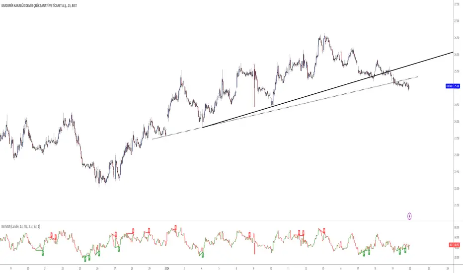
VARGAS"VARGAS" is an indicator that can be used in all timeframes on charts in the stock, crypto, and commodity markets. It allows trades to be opened according to the intersections of moving averages in different time periods.
It is an indicator using weighted moving averages. Using a weighted moving average has the following benefits for traders:
1) Precision and Smoothness: The WMA typically gives more weight to recent prices and therefore reacts faster to more recent data. This helps you catch price movements faster and recognize trend changes faster. On the other hand, the WMA is smoother than the simple moving average (SMA), which makes it less likely to generate false signals.
2) Trend Identification: The WMA is used to identify and analyze price trends. It is especially important for traders who want to track short-term movements. The WMA is used to assess the direction and strength of the trend.
3) Trading Signals: The WMA is used as part of various trading strategies. It is especially used in moving average crossover strategies. For example, a short-term WMA crossing the long-term WMA to the upside can be considered a buy signal, while a reversal can be interpreted as a sell signal.
4) Adaptability to Volatility: WMA can adapt to volatility by changing weighting factors. Investors can adopt a more flexible approach by assigning different weights based on market conditions and asset classes.
5) Data Correction: WMA can be helpful in reducing data noise. A single large price fluctuation can cause the SMA to be more affected, while the WMA reduces the impact of these fluctuations.
In our VARGAS coding, the intersection times of the 9-day and 15-day weighted moving averages allow us to decide the direction of the trend. The green and red cloud areas following the price candles make the strategy easy for the user to follow.
At the intersection between the 9-day weighted moving average and the 15-day weighted moving average, we can use buy and sell signals as follows:
If the 9-day weighted moving average crosses the 15-day weighted moving average upwards, buy,
Sell if the 9-day weighted moving average crosses the 15-day weighted moving average downwards.
Within the scope of this strategy, GOLDEN CROSS and DEATH CROSS intersections, which guide us for trend changes, are also included in the coding. Thus, it is aimed to add strength to our WMA 9 and WMA 15 intersection strategy as an idea.
VARGAS indicator gives better results for longer periods of 4 hours and above. As the time period increases, the probability of correct results will increase.
**
"VARGAS" hisse senedi, kripto, ve emtia piyasalarındaki grafiklerde her türlü zaman diliminde kullanılabilen bir indikatördür. Farklı zaman periyotlarındaki hareketli ortalamaların kesişimlerine göre işlem açılmasını sağlar.
Ağırlıklı hareketli ortalamalar kullanılarak hazırlanmış bir göstergedir. Ağırlıklı hareketli ortalama kullanmanın yatırımcılara aşağıdaki gibi faydaları bulunmaktadır:
1) Duyarlılık ve Pürüzsüzlük: WMA, tipik olarak son dönem fiyatlarına daha fazla ağırlık verir ve bu nedenle daha güncel verilere daha hızlı tepki verir. Bu, fiyat hareketlerini daha hızlı yakalamanıza ve daha hızlı trend değişikliklerini tanımanıza yardımcı olur. Diğer yandan, WMA, basit hareketli ortalamaya (SMA) göre daha pürüzsüzdür, bu da yanlış sinyal üretme olasılığını azaltır.
2) Trend Belirleme: WMA, fiyat trendlerini belirlemek ve analiz etmek için kullanılır. Özellikle kısa vadeli hareketleri izlemek isteyen yatırımcılar için önemlidir. WMA, trendin yönünü ve gücünü değerlendirmek için kullanılır.
3) Ticaret Sinyalleri: WMA, çeşitli ticaret stratejilerinin bir parçası olarak kullanılır. Özellikle hareketli ortalama crossover stratejilerinde kullanılır. Örneğin, kısa vadeli WMA'nın uzun vadeli WMA'yı yukarı yönlü kesmesi bir alım sinyali olarak kabul edilebilir, tersine dönmesi ise bir satış sinyali olarak yorumlanabilir.
4) Volatiliteye Uyarlanabilirlik: WMA, ağırlıklandırma faktörlerini değiştirerek volatiliteye uyum sağlayabilir. Yatırımcılar, piyasa koşullarına ve varlık sınıflarına göre farklı ağırlıklar atayarak daha esnek bir yaklaşım benimseyebilirler.
5) Veri Düzeltme: WMA, veri gürültüsünü azaltmada yardımcı olabilir. Tek bir büyük fiyat dalgalanması, SMA'nın daha fazla etkilenmesine neden olabilirken, WMA bu dalgalanmaların etkisini azaltır.
VARGAS isimli kodlamamızda ise 9 günlük ve 15 günlük ağırlıklı hareketli ortalamaların kesişme zamanları trendin yönüne karar vermemizi sağlar. Fiyat mumlarını takip eden yeşil ve kırmızı bulut alanları stratejinin kullanıcı tarafından kolaylıkla takip edilmesini sağlamaktadır.
9 Günlük Ağırlıklı hareketli ortalama, 15 Günlük Ağırlıklı hareketli ortalama arasındaki kesişimde al ve sat sinyallerini şu şekilde kullanabiliriz:
Eğer 9 günlük ağırlıklı hareketli ortalama 15 günlük ağırlıklı hareketli ortalamayı yukarı doğru kesiyorsa al,
Eğer 9 günlük ağırlıklı hareketli ortalama, 15 günlük ağırlıklı hareketli ortalamayı aşağı doğru keserse sat.
Bu strateji kapsamında trend değişimleri için bizlere yön veren GOLDEN CROSS ve DEATH CROSS kesişimleri de kodlamanın içerisinde dahil edilmiştir. Böylelikle WMA 9 ve WMA 15 kesişim stratejimize fikir olarak güç katması hedeflenmiştir.
VARGAS indikatörü 4 saat ve üzeri daha uzun periyotlarda daha iyi sonuçlar vermektedir. Zaman periyodu büyüdükçe doğru sonuç verme olasılığı artacaktır.
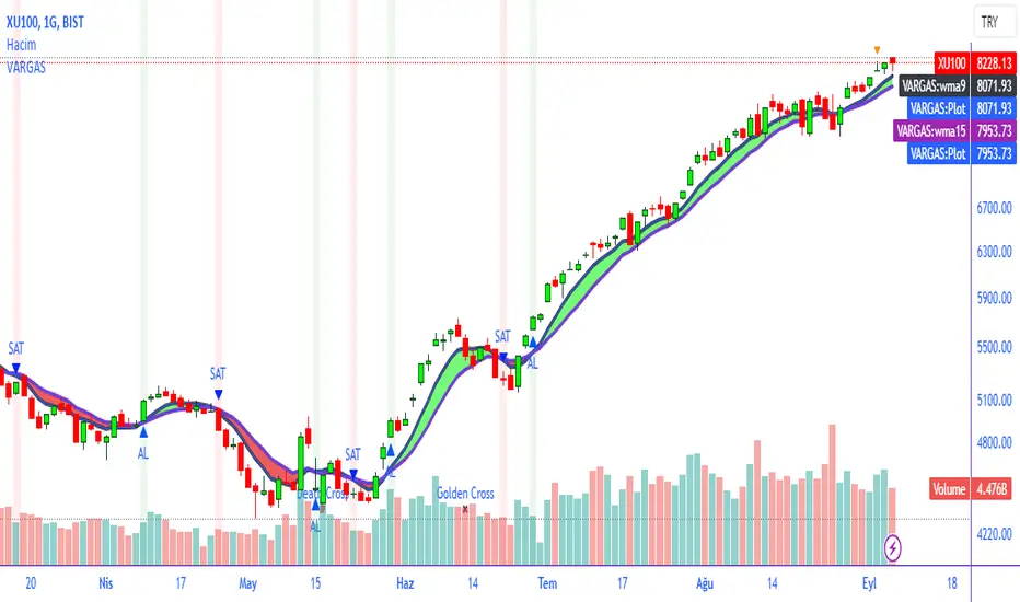
Adaptive Trend SelectorThe Adaptive Trend Selector is a comprehensive trend-following tool designed to automatically identify the optimal moving average crossover strategy. It features adjustable parameters and an integrated backtester that delivers institutional-grade insights into the recommended strategy. The model continuously adapts to new data in real time by evaluating multiple moving average combinations, determining the best performing lengths, and presenting the backtest results in a clear, color-coded table that benchmarks performance against the buy-and-hold strategy.
At its core, the model systematically backtests a wide range of moving average combinations to identify the configuration that maximizes the selected optimization metric. Users can choose to optimize for absolute returns or risk-adjusted returns using the Sharpe, Sortino, or Calmar ratios. Alternatively, users can enable manual optimization to test custom fast and slow moving average lengths and view the corresponding backtest results. The label displays the Compounded Annual Growth Rate (CAGR) of the strategy, with the buy-and-hold CAGR in parentheses for comparison. The table presents the backtest results based on the fast and slow lengths displayed at the top:
Sharpe = CAGR per unit of standard deviation.
Sortino = CAGR per unit of downside deviation.
Calmar = CAGR relative to maximum drawdown.
Max DD = Largest peak-to-trough decline in value.
Beta (β) = Return sensitivity relative to buy-and-hold.
Alpha (α) = Excess annualized risk-adjusted returns.
Win Rate = Ratio of profitable trades to total trades.
Profit Factor = Total gross profit per unit of losses.
Expectancy = Average expected return per trade.
Trades/Year = Average number of trades per year.
This indicator is designed with flexibility in mind, enabling users to specify the start date of the backtesting period and the preferred moving average strategy. Supported strategies include the Exponential Moving Average (EMA), Simple Moving Average (SMA), Wilder’s Moving Average (RMA), Weighted Moving Average (WMA), and Volume-Weighted Moving Average (VWMA). To minimize overfitting, users can define constraints such as a minimum and maximum number of trades per year, as well as an optional optimization margin that prioritizes longer, more robust combinations by requiring shorter-length strategies to exceed this threshold. The table follows an intuitive color logic that enables quick performance comparison against buy-and-hold (B&H):
Sharpe = Green indicates better than B&H, while red indicates worse.
Sortino = Green indicates better than B&H, while red indicates worse.
Calmar = Green indicates better than B&H, while red indicates worse.
Max DD = Green indicates better than B&H, while red indicates worse.
Beta (β) = Green indicates better than B&H, while red indicates worse.
Alpha (α) = Green indicates above 0%, while red indicates below 0%.
Win Rate = Green indicates above 50%, while red indicates below 50%.
Profit Factor = Green indicates above 2, while red indicates below 1.
Expectancy = Green indicates above 0%, while red indicates below 0%.
In summary, the Adaptive Trend Selector is a powerful tool designed to help investors make data-driven decisions when selecting moving average crossover strategies. By optimizing for risk-adjusted returns, investors can confidently identify the best lengths using institutional-grade metrics. While results are based on the selected historical period, users should be mindful of potential overfitting, as past results may not persist under future market conditions. Since the model recalibrates to incorporate new data, the recommended lengths may evolve over time.

40 Ticker Cross-Sectional Z-Scores [BackQuant]40 Ticker Cross-Sectional Z-Scores
BackQuant’s 40 Ticker Cross-Sectional Z-Scores is a powerful portfolio management strategy that analyzes the relative performance of up to 40 different assets, comparing them on a cross-sectional basis to identify the top and bottom performers. This indicator computes Z-scores for each asset based on their log returns and evaluates them relative to the mean and standard deviation over a rolling window. The Z-scores represent how far an asset's return deviates from the average, and these values are used to rank the assets, allowing for dynamic asset allocation based on performance.
By focusing on the strongest-performing assets and avoiding the weakest, this strategy aims to enhance returns while managing risk. Additionally, by adjusting for standard deviations, the system offers a risk-adjusted method of ranking assets, making it suitable for traders who want to dynamically allocate capital based on performance metrics rather than just price movements.
Key Features
1. Cross-Sectional Z-Score Calculation:
The system calculates Z-scores for 40 different assets, evaluating their log returns against the mean and standard deviation over a rolling window. This enables users to assess the relative performance of each asset dynamically, highlighting which assets are performing better or worse compared to their historical norms. The Z-score is a useful statistical tool for identifying outliers in asset performance.
2. Asset Ranking and Allocation:
The system ranks assets based on their Z-scores and allocates capital to the top performers. It identifies the top and bottom assets, and traders can allocate capital to the top-performing assets, ensuring that their portfolio is aligned with the best performers. Conversely, the bottom assets are removed from the portfolio, reducing exposure to underperforming assets.
3. Rolling Window for Mean and Standard Deviation Calculations:
The Z-scores are calculated based on rolling means and standard deviations, making the system adaptive to changing market conditions. This rolling calculation window allows the strategy to adjust to recent performance trends and minimize the impact of outdated data.
4. Mean and Standard Deviation Visualization:
The script provides real-time visualizations of the mean (x̄) and standard deviation (σ) of asset returns, helping traders quickly identify trends and volatility in their portfolio. These visual indicators are useful for understanding the current market environment and making more informed allocation decisions.
5. Top & Bottom Performer Tables:
The system generates tables that display the top and bottom performers, ranked by their Z-scores. Traders can quickly see which assets are outperforming and underperforming. These tables provide clear and actionable insights, helping traders make informed decisions about which assets to include in their portfolio.
6. Customizable Parameters:
The strategy allows traders to customize several key parameters, including:
Rolling Calculation Window: Set the window size for the rolling mean and standard deviation calculations.
Top & Bottom Tickers: Choose how many of the top and bottom assets to display and allocate capital to.
Table Orientation: Select between vertical or horizontal table formats to suit the user’s preference.
7. Forward Test & Out-of-Sample Testing:
The system includes out-of-sample forward tests, ensuring that the strategy is evaluated based on real-time performance, not just historical data. This forward testing approach helps validate the robustness of the strategy in dynamic market conditions.
8. Visual Feedback and Alerts:
The system provides visual feedback on the current asset rankings and allocations, with dynamic labels and plots on the chart. Additionally, users receive alerts when allocations change, keeping them informed of important adjustments.
9. Risk Management via Z-Scores and Std Dev:
The system’s approach to asset selection is based on Z-scores, which normalize performance relative to the historical mean. By incorporating standard deviation, it accounts for the volatility and risk associated with each asset. This allows for more precise risk management and portfolio construction.
10. Note on Mean Reversion Strategy:
If you take the inverse of the signals provided by this indicator, the strategy can be used for mean-reversion rather than trend-following. This would involve buying the underperforming assets and selling the outperforming ones. However, it's important to note that this approach does not work well with highly correlated assets, as the relationship between the assets could result in the same directional movement, undermining the effectiveness of the mean-reversion strategy.
References
www.uts.edu.au
onlinelibrary.wiley.com
www.cmegroup.com
Final Thoughts
The 40 Ticker Cross-Sectional Z-Scores strategy offers a data-driven approach to portfolio management, dynamically allocating capital based on the relative performance of assets. By using Z-scores and standard deviations, this strategy ensures that capital is directed to the strongest performers while avoiding weaker assets, ultimately improving the risk-adjusted returns of the portfolio. Whether you’re focused on trend-following or looking to explore mean-reversion strategies, this flexible system can be tailored to suit your investment goals.
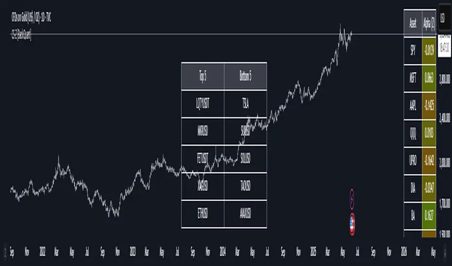
Auto Fib Retracement with Buy/SellKey Features of the Advanced Script:
Multi-Timeframe (MTF) Analysis:
We added an input for the higher timeframe (higher_tf), where the trend is checked on a higher timeframe to confirm the primary trend direction.
Complex Trend Detection:
The trend is determined not only by the current timeframe but also by the trend on the higher timeframe, giving a more comprehensive and reliable signal.
Dynamic Fibonacci Levels:
Fibonacci lines are plotted dynamically, extending them based on price movement, with the Fibonacci retracement drawn only when a trend is identified.
Background Color & Labels:
A background color is added to give a clear indication of the trend direction. Green for uptrend, red for downtrend. It makes it visually easier to understand the current market structure.
"Buy" or "Sell" labels are shown directly on the chart to mark possible entry points.
Strategy and Backtesting:
The script includes strategy commands (strategy.entry and strategy.exit), which allow for backtesting the strategy in TradingView.
Stop loss and take profit conditions are added (loss=100, profit=200), which can be adjusted according to your preferences.
Next Steps:
Test with different timeframes: Try changing the higher_tf to different timeframes (like "60" or "240") and see how it affects the trend detection.
Adjust Fibonacci settings: Modify how the Fibonacci levels are calculated or add more Fibonacci levels like 38.2%, 61.8%, etc.
Optimize Strategy Parameters: Fine-tune the entry/exit logic by adjusting stop loss, take profit, and other strategy parameters.
This should give you a robust foundation for creating advanced trend detection strategies
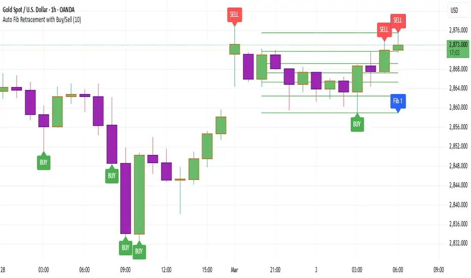
Strategy: Candlestick Wick Analysis with Volume Conditions
This strategy focuses on analyzing the wicks (or shadows) of candlesticks to identify potential trading opportunities based on candlestick structure and volume. Based on these criteria, it places stop orders at the extremities of the wicks when certain conditions are met, thus increasing the chances of capturing significant price movements.
Trading Criteria
Volume Conditions:
The strategy checks if the volume of the current candle is higher than that of the previous three candles. This ensures that the observed price movement is supported by significant volume, increasing the probability that the price will continue in the same direction.
Wick Analysis:
Upper Wick:
If the upper wick of a candle represents more than 90% of its body size and is longer than the lower wick, this indicates that the price tested a resistance level before pulling back.
Order Placement: In this case, a Buy Stop order is placed at the upper extremity of the wick. This means that if the price rises back to this level, the order will be triggered, and the trader will take a buy position.
SL Management: A stop-loss is then placed below the lowest point of the same candle. This protects the trader by limiting losses if the price falls back after the order is triggered.
Lower Wick:
If the lower wick of a candle is longer than the upper wick and represents more than 90% of its body size, this indicates that the price tested a support level before rising.
Order Placement: In this case, a Sell Stop order is placed at the lower extremity of the wick. Thus, if the price drops back to this level, the order will be triggered, and the trader will take a sell position.
SL Management: A stop-loss is then placed above the highest point of the same candle. This ensures risk management by limiting losses if the price rebounds upward after the order is triggered.
Strategy Advantages
Responsiveness to Price Movements: The strategy is designed to detect significant price movements based on the market's reaction around support and resistance levels. By placing stop orders directly at the wick extremities, it allows capturing strong movements in the direction indicated by the candles.
Securing Positions: Using stop-losses positioned just above or below key levels (wicks) provides better risk management. If the market doesn't move as expected, the position is automatically closed with a limited loss.
Clear Visual Indicators: Symbols are displayed on the chart at the points where orders have been placed, making it easier to understand trading decisions. This helps to quickly identify the support or resistance levels tested by the price, as well as potential entry points.
Conclusion
The strategy is based on the idea that large wicks signal areas where buyers or sellers have tested significant price levels before temporarily retreating. By placing stop orders at the extremities of these wicks, the strategy allows capturing price movements when they confirm, while limiting risks through strategically placed stop-losses. It thus offers a balanced approach between capturing potential profit and managing risk.
This description emphasizes the idea of capturing significant market movements with stop orders while providing a clear explanation of the logic and risk management. It’s tailored for publication on TradingView and highlights the robustness of the strategy.